library(simulateGP)
library(systemfit)
#> Loading required package: Matrix
#> Loading required package: car
#> Loading required package: carData
#> Loading required package: lmtest
#> Loading required package: zoo
#>
#> Attaching package: 'zoo'
#> The following objects are masked from 'package:base':
#>
#>     as.Date, as.Date.numeric
#>
#> Please cite the 'systemfit' package as:
#> Arne Henningsen and Jeff D. Hamann (2007). systemfit: A Package for Estimating Systems of Simultaneous Equations in R. Journal of Statistical Software 23(4), 1-40. http://www.jstatsoft.org/v23/i04/.
#>
#> If you have questions, suggestions, or comments regarding the 'systemfit' package, please use a forum or 'tracker' at systemfit's R-Forge site:
#> https://r-forge.r-project.org/projects/systemfit/
The Mendelian randomisation statistical method aims to estimate the causal effect of some exposure \(x\) on some outcome \(y\) using a genetic instrumental variable for the exposure, \(g\). The assumptions of the model are that
- \(g\) associates with \(x\)
- \(g\) is independent of any confounders of \(x\) and \(y\)
- \(g\) only associates with \(y\) via \(x\)
A DAG representing the assumptions is below:
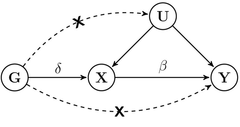
mrdag
We can simulate individual level data according to this DAG
- Simulate some genetic or confounding variables
- Simulate exposures that are influenced by (1)
- Simulate the outcomes that are influenced by (1) and (2)
- Obtain MR estimate using two-stage least squares
Here is how to do 1-3:
# Set causal effect of x on y
beta_xy <- -0.3

# Set number of instruments for x
nsnp <- 3

# Set number of individuals to simulate
nid <- 10000

# Set variance explained in x by the instruments
rsq_gx <- 0.05

# Generate a confounder
u <- rnorm(nid)

# Generate genotypes with allele frequencies of 0.5
g <- make_geno(nid=nid, nsnp=nsnp, af=0.5)

# These SNPs instrument some exposure, and together explain 5% of the variance
effs <- choose_effects(nsnp=nsnp, totvar=rsq_gx)

# Create X - influenced by snps and the confounder
x <- make_phen(effs=c(effs, 0.3), indep=cbind(g, u))
Check that the SNPs explain 5% of the variance in x
Create Y, which is negatively influenced by x and positively influenced by the confounder
We now have an X and Y, and the genotypes. To perform 2-stage least
squares MR on this we can use the systemfit package.
summary(systemfit::systemfit(y ~ x, method="2SLS", inst = ~ g))
#>
#> systemfit results
#> method: 2SLS
#>
#>            N   DF     SSR  detRCov   OLS-R2 McElroy-R2
#> system 10000 9998 9634.32 0.963625 0.036471   0.036471
#>
#>         N   DF     SSR      MSE     RMSE       R2   Adj R2
#> eq1 10000 9998 9634.32 0.963625 0.981644 0.036471 0.036375
#>
#> The covariance matrix of the residuals
#>          eq1
#> eq1 0.963625
#>
#> The correlations of the residuals
#>     eq1
#> eq1   1
#>
#>
#> 2SLS estimates for 'eq1' (equation 1)
#> Model Formula: y ~ x
#> Instruments: ~g
#>
#>                 Estimate   Std. Error  t value   Pr(>|t|)
#> (Intercept)  4.09846e-17  9.81644e-03  0.00000          1
#> x           -3.19712e-01  4.11100e-02 -7.77698 8.2157e-15 ***
#> ---
#> Signif. codes:  0 '***' 0.001 '**' 0.01 '*' 0.05 '.' 0.1 ' ' 1
#>
#> Residual standard error: 0.981644 on 9998 degrees of freedom
#> Number of observations: 10000 Degrees of Freedom: 9998
#> SSR: 9634.32414 MSE: 0.963625 Root MSE: 0.981644
#> Multiple R-Squared: 0.036471 Adjusted R-Squared: 0.036375
Compare against confounded observational estimate
summary(lm(y ~ x))
#>
#> Call:
#> lm(formula = y ~ x)
#>
#> Residuals:
#>     Min      1Q  Median      3Q     Max
#> -4.0502 -0.6585 -0.0084  0.6559  4.1172
#>
#> Coefficients:
#>               Estimate Std. Error t value Pr(>|t|)
#> (Intercept)  3.087e-17  9.762e-03    0.00        1
#> x           -2.169e-01  9.763e-03  -22.22   <2e-16 ***
#> ---
#> Signif. codes:  0 '***' 0.001 '**' 0.01 '*' 0.05 '.' 0.1 ' ' 1
#>
#> Residual standard error: 0.9762 on 9998 degrees of freedom
#> Multiple R-squared:  0.04704,    Adjusted R-squared:  0.04695
#> F-statistic: 493.6 on 1 and 9998 DF,  p-value: < 2.2e-16