Getting Started with kinshipmakr
2025-10-12
kinshipmakr.RmdIntroduction
The kinshipmakr package provides tools for simulating
and analyzing pedigree data. It includes functions for generating
multi-generational pedigrees with realistic mating patterns, calculating
kinship coefficients, and analyzing pedigree structures.
Installation
You can install the package from GitHub:
# install.packages("remotes")
remotes::install_github("yourusername/kinshipmakr")
Load the package:
library(kinshipmakr)Simulating a Pedigree
Let’s start by simulating a small pedigree with 10 founders and 3 generations plus the founders:
# Set random seed for reproducibility
set.seed(123)

# Simulate a pedigree
ped <- simulate_pedigree(
  n_founders = 10,
  n_generations = 3,
  offspring_lambda = 2,
  sex_ratio = 0.5
)

# View the first few rows
head(ped)
#>   id mother father sex generation
#> 1  1      0      0   F          0
#> 2  2      0      0   M          0
#> 3  3      0      0   F          0
#> 4  4      0      0   M          0
#> 5  5      0      0   M          0
#> 6  6      0      0   F          0
The pedigree data frame contains the following columns: -
id: Unique identifier for each individual -
mother: ID of the individual’s mother (0 for founders) -
father: ID of the individual’s father (0 for founders) -
sex: Sex of the individual (“F” or “M”) -
generation: Generation number (0 for founders)
Analyzing Pedigree Structure
We can get a summary of the pedigree structure using the
pedigree_summary function:
pedigree_summary(ped)
#> Pedigree Summary
#> ================
#> Total individuals: 38
#>
#> Individuals per generation:
#>
#>  0  1  2  3
#> 10  9 11  8
#>
#> Sex distribution:
#>
#>  F  M
#> 18 20
This gives us information about: - Total number of individuals - Distribution across generations - Sex distribution
We can also get a list of ancestors for a specific individual:
get_ancestors(id=15, ped)
#> [1] 6 8
and descendents:
get_descendants(id=5, ped)
#> $descendants
#> [1] 13 20 21 31 32 33 34
#>
#> $generation_map
#> 13 20 21 31 32 33 34
#>  1  2  2  3  3  3  3
Calculating Kinship Coefficients
The kinship coefficient between two individuals is the probability
that a randomly chosen allele from one individual is identical by
descent to a randomly chosen allele from the other individual at the
same locus. We can calculate these coefficients using the
calculate_kinship function:
# Calculate kinship matrix
kinship_matrix <- calculate_kinship(ped)

# View a subset of the matrix
kinship_matrix[1:5, 1:5]
#>     1   2   3   4   5
#> 1 0.5 0.0 0.0 0.0 0.0
#> 2 0.0 0.5 0.0 0.0 0.0
#> 3 0.0 0.0 0.5 0.0 0.0
#> 4 0.0 0.0 0.0 0.5 0.0
#> 5 0.0 0.0 0.0 0.0 0.5
The diagonal elements (i,i) represent the inbreeding coefficient + 0.5 for individual i. Off-diagonal elements (i,j) represent the kinship coefficient between individuals i and j.
Example Analyses
Let’s perform some example analyses with our simulated pedigree:
1. Finding Highly Related Pairs
# Function to find pairs with high kinship coefficients
find_related_pairs <- function(kinship_matrix, threshold = 0.125) {
  pairs <- which(kinship_matrix > threshold &
                upper.tri(kinship_matrix),
                arr.ind = TRUE)
  if(nrow(pairs) == 0) return(NULL)

  data.frame(
    id1 = rownames(kinship_matrix)[pairs[,1]],
    id2 = colnames(kinship_matrix)[pairs[,2]],
    kinship = kinship_matrix[pairs]
  )
}

# Find related pairs
related_pairs <- find_related_pairs(kinship_matrix)
head(related_pairs)
#>   id1 id2 kinship
#> 1   3  11    0.25
#> 2   4  11    0.25
#> 3   3  12    0.25
#> 4   4  12    0.25
#> 5  11  12    0.25
#> 6   1  13    0.25
2. Analyzing Inbreeding Coefficients
# Get inbreeding coefficients (diagonal elements - 0.5)
inbreeding <- diag(kinship_matrix) - 0.5

# Summary statistics of inbreeding coefficients
summary(inbreeding)
#>    Min. 1st Qu.  Median    Mean 3rd Qu.    Max.
#> 0.00000 0.00000 0.00000 0.03289 0.03125 0.18750

# Plot distribution of inbreeding coefficients
hist(inbreeding,
     main = "Distribution of Inbreeding Coefficients",
     xlab = "Inbreeding Coefficient",
     breaks = 20)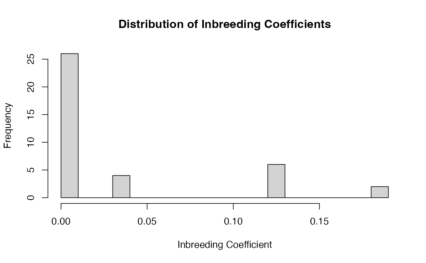
Check if the kinship matrix is positive definite (invertible)
4. Visualizing Kinship Relationships
The package provides a function to visualize kinship matrices as heatmaps. This function automatically handles large pedigrees by sampling if necessary, and includes generation information as color annotations:
plot_kinship(kinship_matrix, ped)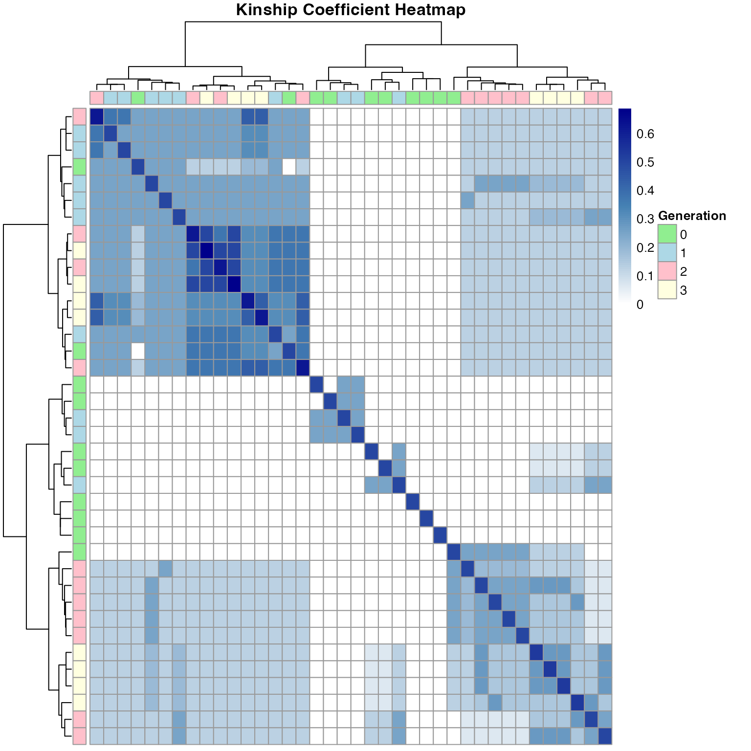
We can also customize the visualization. Let’s create a larger pedigree to demonstrate the sampling feature
large_ped <- simulate_pedigree(
  n_founders = 500,
  n_generations = 3,
  offspring_lambda = 3
)
pedigree_summary(large_ped)
#> Pedigree Summary
#> ================
#> Total individuals: 2157
#>
#> Individuals per generation:
#>
#>   0   1   2   3
#> 500 490 549 618
#>
#> Sex distribution:
#>
#>    F    M
#> 1083 1074
large_kinship <- calculate_kinship(large_ped)

# Custom colors for a different look
custom_colors <- grDevices::colorRampPalette(c("yellow", "red", "darkred"))(100)
gen_colors <- c("0" = "lightgreen", "1" = "lightblue",
                "2" = "pink", "3" = "lightyellow")

# Plot with custom settings
plot_kinship(large_kinship, large_ped,
            max_size = 75,  # Limit to 75 individuals
            colors = custom_colors,
            gen_colors = gen_colors,
            cluster = TRUE)
#> Sampling 75 individuals from 2157 total for visualization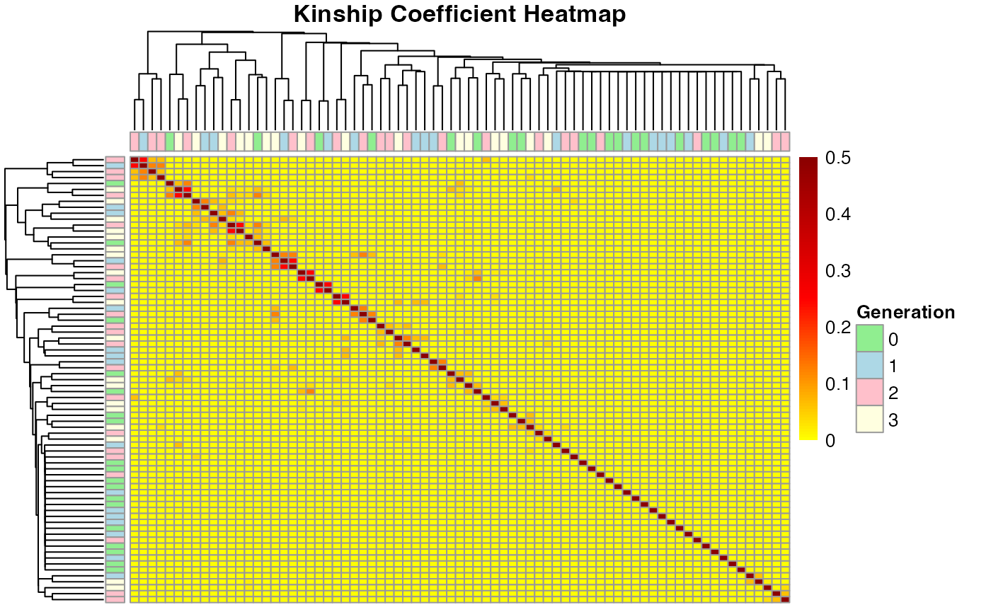
Check if the kinship matrix is invertible:
# Check invertibility using RArpack (much faster than eigen())
result <- check_invertible(large_kinship)
result
#> $is_invertible
#> [1] TRUE
#>
#> $condition_number
#> [1] 241.83
#>
#> $min_eigenvalue
#> [1] 0.03474824
#>
#> $max_eigenvalue
#> [1] 8.403168
The condition number gives us information about the numerical stability of matrix operations. A high condition number (> 1e6) indicates that the matrix is ill-conditioned and numerical computations might be unstable.
t1 <- Sys.time()
large_ped <- simulate_pedigree(
  n_founders = 1000,
  n_generations = 3,
  offspring_lambda = 3
)
pedigree_summary(large_ped)
#> Pedigree Summary
#> ================
#> Total individuals: 4338
#>
#> Individuals per generation:
#>
#>    0    1    2    3
#> 1000 1055 1090 1193
#>
#> Sex distribution:
#>
#>    F    M
#> 2186 2152
Sys.time() - t1
#> Time difference of 1.17999 secs

t2 <- Sys.time()
large_kinship <- calculate_kinship(large_ped)
Sys.time() - t2
#> Time difference of 0.3421409 secs
Kinships from larger pedigrees
Sparse matrices can be used to handle larger pedigrees efficiently.
ped <- simulate_pedigree(
  n_founders = 1000,
  n_generations = 5,
  offspring_lambda = 3
)

pedigree_summary(ped)
#> Pedigree Summary
#> ================
#> Total individuals: 7125
#>
#> Individuals per generation:
#>
#>    0    1    2    3    4    5
#> 1000 1060 1176 1248 1237 1404
#>
#> Sex distribution:
#>
#>    F    M
#> 3627 3498
t1 <- Sys.time()
k1 <- calculate_kinship(ped, sparse=FALSE)  # Dense matrix
Sys.time() - t1
#> Time difference of 0.6178398 secs
object.size(k1) |> format(units="MB")
#> [1] "388.2 Mb"
t2 <- Sys.time()
k2 <- calculate_kinship(ped, sparse=TRUE)   # Sparse matrix
Sys.time() - t2
#> Time difference of 0.823745 secs
object.size(k2) |> format(units="MB")
#> [1] "56.1 Mb"
Using the rARPACK library on sparse matrices is much faster and memory efficient:
check_invertible(k2)
#> $is_invertible
#> [1] TRUE
#>
#> $condition_number
#> [1] 396.5987
#>
#> $min_eigenvalue
#> [1] 0.03529218
#>
#> $max_eigenvalue
#> [1] 13.99683