flowchart TB
    C["C<br/>Shared family environment"]
    GP["G_parent<br/>Parental genetic score"]
    ZP["Z_parent<br/>Parental phenotype"]
    GO["G_off<br/>Offspring genetic score"]
    EO["E_off<br/>Offspring environment"]
    ZO["Z_off<br/>Offspring phenotype"]
    WO["W_off<br/>MR fitness outcome"]
    EF["E_family<br/>Mean offspring environment"]
    WP["W_parent<br/>Price reproductive contribution"]

    C -->|rho| GP
    GP -->|alpha| ZP
    C -->|0.30| ZP
    GP -->|1| GO
    ZP -->|eta| EO
    C -->|0.40| EO
    GO -->|alpha| ZO
    EO -->|beta_env| ZO
    ZO -->|theta| WO
    EO -->|psi| WO
    C -->|gamma| WO
    EO -->|mean across siblings| EF
    EF -->|psi| WP
    ZP -->|theta| WP
    C -->|gamma| WP

    classDef family fill:#e8f0fe,stroke:#3569a8,color:#172b4d;
    classDef offspring fill:#fff1df,stroke:#b66b13,color:#53350d;
    classDef outcome fill:#e3f3e8,stroke:#34764b,color:#163f26;
    classDef contribution fill:#f0e8fa,stroke:#8051a8,color:#43265b;
    class C,GP,ZP family;
    class GO,EO,ZO offspring;
    class WO outcome;
    class EF,WP contribution;
Background
Does the difference between population and within-family Mendelian randomisation (MR) relate to transmission bias in the Price equation?
\[ b_{\mathrm{population}} = b_{\mathrm{within\text{-}family}} + b_{\mathrm{residual}}. \]
This MR decomposition defines the residual by subtraction. The Price equation instead decomposes change in a population mean into selection and transmission:
\[ \Delta \bar z = \underbrace{\frac{\operatorname{Cov}_N(w_i,z_i)}{\bar w}}_{\text{selection}} + \underbrace{\frac{\mathbb E_i[w_i\Delta z_i]}{\bar w}}_{\text{transmission}}. \]
Here \(i\) indexes parents, \(w_i\) is their reproductive contribution, and \(\Delta z_i\) is the mean phenotype difference between their descendants and themselves. Both terms use the same normalisation by mean reproductive contribution. The covariance is a population covariance, with denominator \(N\), rather than R’s sample covariance with denominator \(N-1\). These definitions give an exact identity for the specified ancestor–descendant mapping. Frank (1997) derives the identity and the assignment of descendant contributions.
The two decompositions concern different quantities: MR estimates fitness change per unit phenotype, whereas the Price terms measure phenotype change between generations. A numerical correspondence between their components is therefore not an identity. The simulation below explores how shared pathways affect both.
Simulation setup
Each family has one representative parent and two sampled offspring. This is an illustrative family genetic score model: offspring scores vary around the parental score, rather than following an explicit two-parent, diploid inheritance model. The offspring fitness outcome is a continuous linear index, which can be negative; it is not an offspring count or a survival probability.
The parameters distinguish the direct phenotype effect (theta), parental effects on offspring environment (eta), the direct environment effect on offspring fitness (psi), the shared family environment effect on fitness (gamma), and the correlation of parental genotype with shared environment (rho). In particular, setting rho = 0 removes that initial correlation but leaves the parental genotype → parental phenotype → offspring environment pathway.
Data-generating graph
Figure 1 shows the dependencies in the simulation. Each offspring has its own G_off, E_off, Z_off, and W_off, while C, G_parent, and Z_parent are shared within its family. The family mean of offspring environment enters the separate parental reproductive contribution used by the Price equation.
The C → G_parent arrow records how the code constructs their correlation; it does not assert that environment changes genotype. Setting rho = 0 deletes this dependence while retaining G_parent → Z_parent → E_off. Setting psi = 0 removes both E_off → W_off and E_family → W_parent, while the gamma pathways remain. The E_off → Z_off → W_off pathway also remains because psi controls only the direct environment effect on fitness.
Generate parents and individual offspring
C is the shared family environment. The parental genetic score has unit variance and correlation rho with C. Offspring genetic deviations and individual environmental noise are independent. Under these assumptions, within-family genetic variation provides an instrument for the direct phenotype effect theta.
Parental reproductive contribution is kept positive by a floor at 0.05. It is a modelled contribution to a reweighted descendant cohort, not a realised count: every family supplies the same number of sampled offspring. The family mean of E_off is used only to define this parental contribution. Offspring phenotypes remain individual observations for the Price calculation.
simulate_generations <- function(
    n_families = 20000, n_siblings = 2,
    theta = 0.20, eta = 0.50, psi = 0.30, gamma = 0.30,
    rho = 0.50, alpha = 0.50, beta_env = 0.50
) {
  stopifnot(
    length(n_families) == 1L, n_families >= 2,
    n_families == as.integer(n_families),
    length(n_siblings) == 1L, n_siblings >= 2,
    n_siblings == as.integer(n_siblings),
    length(rho) == 1L, is.finite(rho), abs(rho) <= 1
  )

  # Parental genetic and phenotypic variation.
  C <- rnorm(n_families)
  G_parent <- rho * C + sqrt(1 - rho^2) * rnorm(n_families)
  Z_parent <- alpha * G_parent + 0.30 * C +
    rnorm(n_families, sd = 0.7)

  # Each row below represents one offspring, linked to its parent.
  family_id <- rep(seq_len(n_families), each = n_siblings)
  n_offspring <- length(family_id)
  G_off <- G_parent[family_id] + rnorm(n_offspring, sd = 0.7)
  E_off <- eta * Z_parent[family_id] + 0.40 * C[family_id] +
    rnorm(n_offspring, sd = 0.7)
  Z_off <- alpha * G_off + beta_env * E_off +
    rnorm(n_offspring, sd = 0.7)

  # Fitness index used as the MR outcome, not as a Price weight.
  W_off <- 1 + theta * Z_off + psi * E_off +
    gamma * C[family_id] + rnorm(n_offspring, sd = 0.3)

  # Positive parental reproductive contributions used by Price.
  E_family <- family_means(E_off, family_id, n_families)
  W_parent <- pmax(
    1 + theta * Z_parent + psi * E_family + gamma * C +
      rnorm(n_families, sd = 0.2),
    0.05
  )

  list(
    parents = data.frame(
      family_id = seq_len(n_families), C = C,
      G_parent = G_parent, Z_parent = Z_parent, W_parent = W_parent
    ),
    offspring = data.frame(
      family_id = family_id, G_off = G_off, E_off = E_off,
      Z_off = Z_off, W_off = W_off
    )
  )
}
Estimate population and within-family MR
Population MR is a Wald ratio of genotype–fitness and genotype–phenotype associations. Within-family MR uses the same ratio after subtracting family means from all three variables. This removes shared family terms; individual environmental noise remains, but is independent of the within-family genetic instrument in this model. Consequently, the within-family estimator targets theta, with sampling error.
R’s sample covariance is appropriate here because the common \(N-1\) factors cancel within each ratio. The residual captures the difference between the estimators, including sampling variation.
estimate_mr <- function(offspring, n_families) {
  demean <- function(x) {
    means <- family_means(x, offspring$family_id, n_families)
    x - means[offspring$family_id]
  }

  b_population <- with(offspring, cov(G_off, W_off) / cov(G_off, Z_off))
  G_within <- demean(offspring$G_off)
  Z_within <- demean(offspring$Z_off)
  W_within <- demean(offspring$W_off)
  b_withinfamily <- cov(G_within, W_within) / cov(G_within, Z_within)

  list(
    b_population = b_population,
    b_withinfamily = b_withinfamily,
    b_residual = b_population - b_withinfamily
  )
}
Assign each offspring its parent’s reproductive weight
For offspring \(j\) of parent \(i\), we explicitly attach \(w_i\) and \(z_i\) to its row. If parent \(i\) has \(n_i\) sampled offspring, that offspring’s contribution weight is \(a_{ij}=w_i/n_i\). Thus the weights of all sampled offspring of a parent sum to that parent’s total reproductive contribution. With two offspring per family, using \(w_i\) directly gives the same normalised weighted mean because the common factor of two cancels. Dividing by \(n_i\) also handles unequal sampling counts without inadvertently giving more weight to families with more sampled offspring.
The descendant mean and transmission term are computed directly over individual offspring:
\[ \bar z' = \frac{\sum_i\sum_j a_{ij}z_{ij}}{\sum_i w_i}, \qquad T = \frac{\sum_i\sum_j a_{ij}(z_{ij}-z_i)}{\sum_i w_i}. \]
The selection term still compares parents, each counted once. These individual calculations are algebraically equivalent to first averaging offspring phenotypes within each family when the same allocation of parental contribution is used. Averaging was not itself a bias in the original balanced simulation, but the explicit mapping makes the weighting inspectable.
assign_offspring_weights <- function(parents, offspring) {
  stopifnot(!anyDuplicated(parents$family_id))
  parent_index <- match(offspring$family_id, parents$family_id)
  stopifnot(!anyNA(parent_index))
  counts <- tabulate(parent_index, nbins = nrow(parents))
  stopifnot(
    all(counts > 0), all(is.finite(parents$W_parent)),
    all(parents$W_parent >= 0), sum(parents$W_parent) > 0
  )

  offspring$Z_parent <- parents$Z_parent[parent_index]
  offspring$parent_reproductive_weight <- parents$W_parent[parent_index]
  offspring$contribution_weight <-
    offspring$parent_reproductive_weight / counts[parent_index]
  offspring
}
estimate_price <- function(parents, weighted_offspring) {
mean_w <- mean(parents$W_parent)
selection <- cov_population(parents$W_parent, parents$Z_parent) / mean_w
# No averaging of offspring phenotypes: use each offspring's difference.
transmission <- with(weighted_offspring, weighted.mean(
Z_off - Z_parent, contribution_weight
))
delta_z <- with(weighted_offspring, weighted.mean(
Z_off, contribution_weight
)) - mean(parents$Z_parent)
list(
price_selection = selection,
price_transmission = transmission,
delta_z = delta_z,
price_sum = selection + transmission,
price_error = delta_z - (selection + transmission)
)
}Decompose the selection term
Substituting E_family into the parental contribution gives, before the floor at 0.05,
\[ W_{\mathrm{parent}} = 1 + (\theta + \psi\eta)\,Z_{\mathrm{parent}} + (\gamma + 0.40\psi)\,C + \text{noise}, \]
where the noise terms (the sibling mean of offspring environmental noise and the parental contribution noise) are independent of \(Z_{\mathrm{parent}}\). The selection term therefore separates approximately into three parts:
\[ \frac{\operatorname{Cov}_N(w,z)}{\bar w} \approx \underbrace{\frac{\theta\operatorname{Var}_N(z)}{\bar w}}_{\text{direct}} + \underbrace{\frac{\psi\eta\operatorname{Var}_N(z)}{\bar w}}_{\text{parental effect}} + \underbrace{\frac{(\gamma + 0.40\psi)\operatorname{Cov}_N(C,z)}{\bar w}}_{\text{confounding via } C}. \]
The direct part is the selection term implied by the causal effect that within-family MR targets. The parental-effect part arises because a parent’s phenotype changes its offspring’s environment, which in turn raises the parent’s reproductive contribution; within-family MR excludes this pathway because eta acts between families. The confounding part reflects the shared environment’s effects on both phenotype and contribution. \(\operatorname{Var}_N(Z_{\mathrm{parent}})\) does not depend on eta, so eta changes selection only through the parental-effect slope.
The split is exact only for the linear predictor. When psi > 0, increasing eta widens the spread of parental contributions, so the floor binds more often and attenuates the simulated covariance. Finite-sample covariance between the noise and phenotype adds a smaller discrepancy.
decompose_selection <- function(parents, theta, eta, psi, gamma) {
  mean_w <- mean(parents$W_parent)
  var_z <- cov_population(parents$Z_parent, parents$Z_parent)
  # 0.40 is the C -> E_off coefficient in simulate_generations().
  list(
    selection_direct = theta * var_z / mean_w,
    selection_parental = psi * eta * var_z / mean_w,
    selection_confounding = (gamma + 0.40 * psi) *
      cov_population(parents$C, parents$Z_parent) / mean_w
  )
}
Combine the estimators
Both decompositions use the same simulated families, but MR uses offspring fitness as its outcome and Price uses parental reproductive contributions as its weights. These are separate modelled quantities. The Price identity is exact for this weighted cohort; it does not establish that the MR residual estimates transmission or that the weighted change equals the unweighted change among the sampled offspring.
simulate_evolution <- function(
    n_families = 20000, n_siblings = 2,
    theta = 0.20, eta = 0.50, psi = 0.30, gamma = 0.30,
    rho = 0.50, alpha = 0.50, beta_env = 0.50
) {
  generations <- simulate_generations(
    n_families = n_families, n_siblings = n_siblings,
    theta = theta, eta = eta, psi = psi, gamma = gamma,
    rho = rho, alpha = alpha, beta_env = beta_env
  )
  offspring <- assign_offspring_weights(
    generations$parents, generations$offspring
  )
  as.data.frame(c(
    list(theta = theta, eta = eta, psi = psi, rho = rho),
    estimate_mr(offspring, n_families),
    estimate_price(generations$parents, offspring),
    decompose_selection(generations$parents, theta, eta, psi, gamma)
  ))
}

result <- simulate_evolution()
print(round(result, 4))
theta eta psi rho b_population b_withinfamily b_residual price_selection
1 0.2 0.5 0.3 0.5 0.5071 0.204 0.3031 0.5126
price_transmission delta_z price_sum price_error selection_direct
1 -0.0485 0.4641 0.4641 0 0.1925
selection_parental selection_confounding
1 0.1444 0.2279Check the weighting and the Price identity
A small example with unequal numbers of sampled offspring checks the allocation independently of the stochastic model. The parental contributions are 1 and 3, and the offspring phenotypes are 2 for the first parent and 4, 8 for the second. Their contribution weights must be 1, 1.5, 1.5. The descendant mean is then 5, selection is 0.25, transmission is 3.25, and total change is 3.5. The checks also verify invariance to row order and to duplicating a parent’s sampled offspring without changing its phenotype distribution.
check_parents <- data.frame(
  family_id = c(10, 20), Z_parent = c(1, 2), W_parent = c(1, 3)
)
check_offspring <- data.frame(family_id = c(10, 20, 20), Z_off = c(2, 4, 8))
check_weighted <- assign_offspring_weights(check_parents, check_offspring)
check_price <- estimate_price(check_parents, check_weighted)
stopifnot(
  isTRUE(all.equal(check_weighted$contribution_weight, c(1, 1.5, 1.5))),
  isTRUE(all.equal(check_price$price_selection, 0.25)),
  isTRUE(all.equal(check_price$price_transmission, 3.25)),
  isTRUE(all.equal(check_price$delta_z, 3.5)),
  abs(check_price$price_error) < 1e-12
)

reordered_parents <- check_parents[2:1, ]
reordered_offspring <- check_offspring[c(3, 1, 2), ]
duplicated_offspring <- check_offspring[c(1, 2, 3, 2, 3), ]
for (sampled_offspring in list(reordered_offspring, duplicated_offspring)) {
  checked <- estimate_price(reordered_parents, assign_offspring_weights(
    reordered_parents, sampled_offspring
  ))
  stopifnot(isTRUE(all.equal(checked, check_price, tolerance = 1e-12)))
}
stopifnot(abs(result$price_error) < 1e-12)
cat("Offspring allocation and Price identity checks passed.\n")
Offspring allocation and Price identity checks passed.Remove the genotype–environment correlation and the environment–fitness effect
Setting rho = 0 makes parental genotype independent of C. It does not make offspring genotype independent of offspring environment: eta * Z_parent still carries parental genetic effects into E_off. Setting psi = 0 removes the direct E_off → W_off pathway, but leaves gamma * C → W_off. Environment also continues to affect offspring phenotype through beta_env, and hence fitness through theta; that mediated effect is consistent with the MR target.
The model gives an analytic check. Let \(K=\operatorname{Cov}(G_{\mathrm{off}},E_{\mathrm{off}})\) and \(D=\operatorname{Cov}(G_{\mathrm{off}},Z_{\mathrm{off}})\). Since the genetic segregation noise has variance \(0.7^2\),
\[ K = \eta(\alpha + 0.30\rho) + 0.40\rho, \qquad D = \alpha(1+0.7^2) + \beta_{\mathrm{env}}K. \]
Substituting the offspring fitness equation into the population Wald ratio gives
\[ b_{\mathrm{population}} \longrightarrow \theta + \frac{\psi K + \gamma\rho}{D}, \qquad b_{\mathrm{within\text{-}family}} \longrightarrow \theta. \]
These are large-sample targets, not exact finite-sample estimates. At eta = 0.5 with the other defaults, they predict:
| Scenario | Population MR | Within-family MR | MR residual |
|---|---|---|---|
Default (rho = 0.5, psi = 0.3) |
0.505 | 0.200 | 0.305 |
rho = 0 |
0.286 | 0.200 | 0.086 |
psi = 0 |
0.349 | 0.200 | 0.149 |
rho = 0, psi = 0 |
0.200 | 0.200 | 0.000 |
With rho = 0 alone, the residual also vanishes at eta = 0. With psi = 0 alone, increasing eta changes the instrument–phenotype association \(D\), so the remaining bias need not stay constant. With both zero, both MR estimators target theta throughout the eta sweep. None of these restrictions forces the Price transmission term to zero: offspring phenotypes can still differ systematically from parental phenotypes, including through regression toward the mean and environmental transmission.
Compare all four scenarios using the same random draws
Each run resets the seed so parameter comparisons share the underlying random draws. This reduces Monte Carlo noise in differences; the runs are not independent replicates and the plots do not provide uncertainty intervals. The analytic targets help distinguish sampling error from the pathways being removed.
scenarios <- data.frame(
  scenario = c("Default", "rho = 0", "psi = 0", "rho = 0, psi = 0"),
  rho = c(0.5, 0, 0.5, 0),
  psi = c(0.3, 0.3, 0, 0)
)
eta_values <- seq(0, 1, by = 0.1)
results <- do.call(rbind, lapply(seq_len(nrow(scenarios)), function(s) {
  do.call(rbind, lapply(eta_values, function(e) {
    set.seed(123)
    fit <- simulate_evolution(eta = e, rho = scenarios$rho[s], psi = scenarios$psi[s])
    fit$scenario <- scenarios$scenario[s]
    K <- e * (0.5 + 0.30 * fit$rho) + 0.40 * fit$rho
    D <- 0.5 * (1 + 0.7^2) + 0.5 * K
    fit$target_population <- fit$theta + (fit$psi * K + 0.30 * fit$rho) / D
    fit$target_withinfamily <- fit$theta
    fit$target_residual <- fit$target_population - fit$theta
    fit
  }))
}))
stopifnot(all(abs(results$price_error) < 1e-12))

# Display the observed estimates and Price terms at the default eta.
comparison <- results[abs(results$eta - 0.5) < 1e-12, c(
  "scenario", "b_population", "b_withinfamily", "b_residual",
  "price_selection", "price_transmission", "delta_z", "target_population"
)]
knitr::kable(comparison, digits = 3, row.names = FALSE)| scenario | b_population | b_withinfamily | b_residual | price_selection | price_transmission | delta_z | target_population |
|---|---|---|---|---|---|---|---|
| Default | 0.507 | 0.204 | 0.303 | 0.513 | -0.049 | 0.464 | 0.505 |
| rho = 0 | 0.291 | 0.204 | 0.087 | 0.385 | -0.077 | 0.308 | 0.286 |
| psi = 0 | 0.350 | 0.197 | 0.153 | 0.356 | -0.049 | 0.307 | 0.349 |
| rho = 0, psi = 0 | 0.204 | 0.197 | 0.006 | 0.256 | -0.070 | 0.186 | 0.200 |
Compare MR and the Price equation side by side
Each column uses the same parameter setting and simulated cohort: MR estimates are on the top row and Price components are on the bottom row. Columns show the default model, rho = 0, psi = 0, and both zero. Axes are held constant within each row across all four columns. The two rows use different units: MR measures fitness index change per unit phenotype, whereas Price measures change in mean phenotype.
For MR, solid lines are simulated estimates and dotted lines are large-sample targets; the horizontal grey line marks theta = 0.2. For Price, the total change is the sum of selection and transmission, and the horizontal grey line marks zero. The shaded areas stack the direct, parental-effect and confounding parts of selection; where the top of the stack lies above the selection line, the floor on parental contributions is attenuating selection. Even where the MR residual approaches zero, Price transmission can remain nonzero.
Changing psi changes the parental weights as well as the offspring fitness outcome, so it can affect both Price components. Changing eta or rho also changes the parent–offspring phenotype distribution. The curves therefore describe the full specified model, rather than isolating a single causal interpretation of transmission.
library(ggplot2)

plot_mr_price <- function(results, scenarios) {
  settings <- sprintf("rho = %.1f, psi = %.1f", scenarios$rho, scenarios$psi)
  methods <- c("MR", "Price equation")
  setting <- factor(
    settings[match(results$scenario, scenarios$scenario)], levels = settings
  )

  # Stack the requested results columns into long format, one spec row each.
  to_long <- function(spec) {
    long <- do.call(rbind, lapply(seq_len(nrow(spec)), function(i) {
      data.frame(
        setting = setting, eta = results$eta,
        spec[i, setdiff(names(spec), "column"), drop = FALSE],
        value = results[[spec$column[i]]],
        row.names = NULL
      )
    }))
    long$method <- factor(long$method, levels = methods)
    long
  }

  curves <- to_long(data.frame(
    column = c("b_population", "b_withinfamily", "b_residual",
      "target_population", "target_withinfamily", "target_residual",
      "price_selection", "price_transmission", "delta_z"),
    method = rep(methods, c(6, 3)),
    series = c(rep(c("Population", "Within-family", "Residual"), 2),
      "Selection", "Transmission", "Total change"),
    type = c(rep(c("Simulated", "Large-sample target"), each = 3),
      rep("Simulated", 3))
  ))
  curves$series <- factor(curves$series, levels = unique(curves$series))
  curves$type <- factor(curves$type, levels = c("Simulated", "Large-sample target"))

  component_labels <- c("Direct", "Parental effect", "Confounding via C")
  components <- to_long(data.frame(
    column = c("selection_direct", "selection_parental", "selection_confounding"),
    method = "Price equation",
    component = component_labels
  ))
  components$component <- factor(components$component, levels = component_labels)

  reference <- data.frame(
    method = factor(methods, levels = methods),
    yintercept = c(0.2, 0)
  )

  ggplot(curves, aes(eta, value)) +
    # Reverse stacking so the direct part sits at the bottom of the stack.
    geom_area(aes(fill = component), data = components,
      position = position_stack(reverse = TRUE)) +
    geom_hline(aes(yintercept = yintercept), data = reference, colour = "grey70") +
    geom_line(aes(colour = series, linetype = type), linewidth = 0.8) +
    scale_x_continuous(breaks = c(0, 0.5, 1)) +
    scale_linetype_manual(values = c(Simulated = "solid", `Large-sample target` = "dotted")) +
    scale_colour_brewer(palette = "Dark2") +
    scale_fill_grey(start = 0.65, end = 0.92) +
    guides(
      colour = guide_legend(nrow = 2, order = 1),
      linetype = guide_legend(ncol = 1, order = 2),
      fill = guide_legend(ncol = 1, order = 3)
    ) +
    facet_grid(method ~ setting, scales = "free_y", switch = "y") +
    labs(
      x = "Parental phenotype effect on offspring environment (eta)",
      y = NULL, colour = NULL, linetype = NULL, fill = "Selection parts"
    ) +
    theme_bw() +
    theme(strip.placement = "outside", legend.position = "bottom")
}
plot_mr_price(results, scenarios)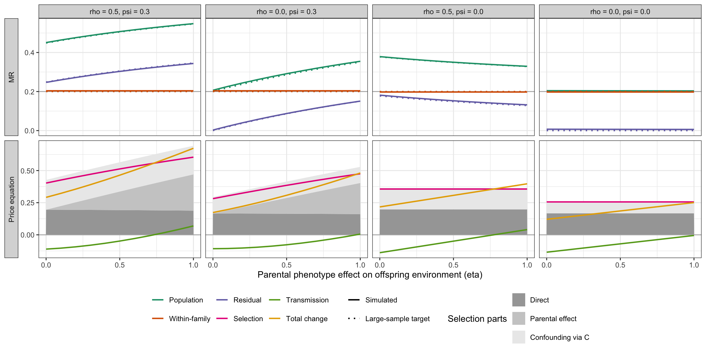
Interpretation
Removing both rho and psi supplies a useful counterexample to identifying the MR residual with Price transmission: the large-sample MR residual is zero, while the Price transmission term need not be. The residual depends on genetic associations with fitness pathways outside the phenotype effect. Price transmission depends on reproductive-contribution-weighted differences between parental and offspring phenotypes. Relating the two would require additional assumptions that connect these estimands and the two fitness definitions.
Checking Frank 1997
dat <- simulate_generations()
offspring <- assign_offspring_weights(
  dat$parents, dat$offspring
)

parents <- dat$parents
str(parents)
'data.frame': 20000 obs. of 5 variables:
$ family_id: int 1 2 3 4 5 6 7 8 9 10 ...
$ C : num -1.863 0.201 0.683 1.222 -1.424 ...
$ G_parent : num -1.808 -0.355 1.024 1.047 -1.975 ...
$ Z_parent : num -1.275 -0.566 0.956 0.995 -0.388 ...
$ W_parent : num 0.05 1.311 1.983 1.591 0.268 ...mean_w <- mean(parents$W_parent)
q_i <- 1/20000
sum(q_i * (parents$W_parent/mean_w - 1) * parents$Z_parent)[1] 0.5078926sum(q_i * parents$W_parent/mean_w * parents$Z_parent) - sum(q_i * parents$Z_parent)[1] 0.5078926(sum(q_i * parents$Z_parent * parents$W_parent) / mean_w - sum(q_i * parents$Z_parent) * sum(q_i * parents$W_parent/mean_w))[1] 0.5078926sum(q_i * parents$W_parent * parents$Z_parent / mean_w - q_i * parents$Z_parent)[1] 0.5078926sum(q_i * parents$W_parent * parents$Z_parent / mean_w) - sum(q_i * parents$Z_parent)[1] 0.5078926sum(q_i * parents$W_parent * parents$Z_parent) / mean_w - sum(q_i * parents$Z_parent)[1] 0.5078926sum(q_i * parents$Z_parent) * sum(q_i * parents$W_parent) / mean_w[1] -0.007540938sum(q_i * parents$Z_parent)[1] -0.007540938Split selection and transmission by source
The sources of MR bias include the direct effect, pleiotropy, population stratification, dynastic effects and assortative mating. Each is a source of covariance between phenotype and fitness. Does each contribute only to the Price selection term, or also to transmission? This section splits both Price terms by the same sources.
With two sampled offspring per parent and contribution weights \(a_{ij} = w_i/2\), the transmission term is exactly
\[ T = \frac{\operatorname{Cov}_N(w, \bar z' - z)}{\bar w} + \overline{(\bar z' - z)}, \]
where \(\bar z'_i\) is the mean phenotype of parent \(i\)’s sampled offspring. Writing the parental contribution as a sum of source terms, \(w = 1 + \sum_s X_s\), each source contributes
\[ S_s = \frac{\operatorname{Cov}_N(X_s, z)}{\bar w}, \qquad T_s = \frac{\operatorname{Cov}_N(X_s, \bar z' - z)}{\bar w} = S_s(\tau_s - 1), \qquad \tau_s = \frac{\operatorname{Cov}_N(X_s, \bar z')}{\operatorname{Cov}_N(X_s, z)}. \]
Here \(\tau_s\) is the transmissibility of source \(s\): the share of its covariance with parental phenotype that reappears as covariance with offspring phenotype. A source with \(\tau_s = 1\) sits entirely in selection. With \(\tau_s < 1\), negative transmission cancels part of its selection; with \(\tau_s > 1\), it adds positive transmission. A source uncorrelated with parental phenotype has no selection part but can still contribute to transmission.
Source terms in this model
| Source | Term in \(W_{\mathrm{parent}}\) |
|---|---|
| Direct | \(\theta Z_{\mathrm{parent}}\) |
| Parental effect | \(\psi\eta Z_{\mathrm{parent}}\) |
| Confounding via \(C\) | \((\gamma + 0.40\psi)C\) |
| Sibling environment | \(\psi(E_{\mathrm{family}} - \eta Z_{\mathrm{parent}} - 0.40C)\) |
| Remainder | Parental noise and the floor at 0.05 |
The sibling environment is the mean of the offspring’s individual environmental noise. It raises the parent’s contribution through psi and the offspring’s phenotype through beta_env. It is therefore independent of parental phenotype but correlated with the parent–offspring difference. The remainder is computed by subtraction, which makes both decompositions exact; the unweighted mean change is added to its transmission part.
The two phenotype sources share one transmissibility: the parent–offspring regression of phenotype,
\[ \tau_Z = \frac{\alpha\operatorname{Cov}(Z_{\mathrm{parent}}, G_{\mathrm{parent}}) + \beta_{\mathrm{env}}\eta\operatorname{Var}(Z_{\mathrm{parent}}) + 0.40\beta_{\mathrm{env}}\operatorname{Cov}(Z_{\mathrm{parent}}, C)}{\operatorname{Var}(Z_{\mathrm{parent}})}. \]
At the default settings, \(\tau_Z\) rises from 0.44 at eta = 0 to 0.94 at eta = 1. Offspring do not inherit the parent’s individual phenotypic noise or the direct C → Z_parent effect, but the eta pathway passes parental phenotype on through the offspring environment. For the shared environment,
\[ \tau_C = \frac{\alpha\rho + \beta_{\mathrm{env}}\{0.40 + \eta\operatorname{Cov}(C, Z_{\mathrm{parent}})\}}{\alpha\rho + 0.30}, \]
which rises from 0.82 to 1.32 at the default settings. The large-sample values at the default settings, before the floor and taking \(\bar w = 1\), are:
| Source | Selection, eta = 0 |
Transmission, eta = 0 |
Selection, eta = 1 |
Transmission, eta = 1 |
|---|---|---|---|---|
| Direct | 0.196 | −0.109 | 0.196 | −0.011 |
| Parental effect | 0.000 | 0.000 | 0.294 | −0.017 |
| Confounding via \(C\) | 0.231 | −0.042 | 0.231 | 0.074 |
| Sibling environment | 0.000 | 0.037 | 0.000 | 0.037 |
| Sum | 0.427 | −0.114 | 0.721 | 0.083 |
Compute the decomposition
decompose_price <- function(parents, offspring, theta, eta, psi, gamma) {
  n <- nrow(parents)
  # family_means() returns values in family ID order.
  stopifnot(identical(parents$family_id, seq_len(n)))
  z <- parents$Z_parent
  z_off <- family_means(offspring$Z_off, offspring$family_id, n)
  e_family <- family_means(offspring$E_off, offspring$family_id, n)
  dz <- z_off - z
  mean_w <- mean(parents$W_parent)

  # 0.40 is the C -> E_off coefficient in simulate_generations().
  terms <- list(
    "Direct" = theta * z,
    "Parental effect" = psi * eta * z,
    "Confounding via C" = (gamma + 0.40 * psi) * parents$C,
    "Sibling environment" = psi * (e_family - eta * z - 0.40 * parents$C)
  )
  terms[["Remainder"]] <- parents$W_parent - 1 - Reduce(`+`, terms)

  out <- data.frame(
    source = names(terms),
    selection = vapply(terms, cov_population, numeric(1), y = z) / mean_w,
    transmission = vapply(terms, cov_population, numeric(1), y = dz) / mean_w,
    row.names = NULL
  )
  # The unweighted mean change belongs to no source; keep the identity exact.
  is_remainder <- out$source == "Remainder"
  out$transmission[is_remainder] <- out$transmission[is_remainder] + mean(dz)
  out
}
The sweep resets the seed before each run, as in sensitivity-analysis, so it reuses the draws behind results. The parts must therefore sum exactly to the Price terms already shown in Figure 2.
price_sources <- do.call(rbind, lapply(seq_len(nrow(scenarios)), function(s) {
  do.call(rbind, lapply(eta_values, function(e) {
    set.seed(123)
    generations <- simulate_generations(
      eta = e, rho = scenarios$rho[s], psi = scenarios$psi[s]
    )
    # theta and gamma are the simulate_generations() defaults.
    parts <- decompose_price(
      generations$parents, generations$offspring,
      theta = 0.20, eta = e, psi = scenarios$psi[s], gamma = 0.30
    )
    cbind(scenario = scenarios$scenario[s], eta = e, parts)
  }))
}))

local({
  totals <- aggregate(
    cbind(selection, transmission) ~ scenario + eta, price_sources, sum
  )
  matched <- merge(
    totals, results[, c("scenario", "eta", "price_selection", "price_transmission")]
  )
  stopifnot(
    nrow(matched) == nrow(results),
    all(abs(matched$selection - matched$price_selection) < 1e-10),
    all(abs(matched$transmission - matched$price_transmission) < 1e-10)
  )
})

# Simulated counterpart of the large-sample table, at the default settings.
local({
  x <- price_sources[
    price_sources$scenario == "Default" & price_sources$eta %in% range(eta_values),
    c("source", "eta", "selection", "transmission")
  ]
  wide <- reshape(x, direction = "wide", idvar = "source", timevar = "eta")
  wide <- rbind(wide, data.frame(source = "Sum", t(colSums(wide[, -1]))))
  knitr::kable(wide, digits = 3, row.names = FALSE, col.names = c(
    "Source", "Selection, eta = 0", "Transmission, eta = 0",
    "Selection, eta = 1", "Transmission, eta = 1"
  ))
})| Source | Selection, eta = 0 | Transmission, eta = 0 | Selection, eta = 1 | Transmission, eta = 1 |
|---|---|---|---|---|
| Direct | 0.196 | -0.108 | 0.188 | -0.010 |
| Parental effect | 0.000 | 0.000 | 0.282 | -0.015 |
| Confounding via C | 0.232 | -0.044 | 0.223 | 0.069 |
| Sibling environment | 0.000 | 0.035 | 0.000 | 0.034 |
| Remainder | -0.025 | 0.005 | -0.089 | -0.010 |
| Sum | 0.403 | -0.111 | 0.604 | 0.069 |
Compare sources across settings
Each row is one source and each column one parameter setting. The total line is the source’s contribution to the change in mean phenotype, \(S_s + T_s\). Where the transmission line sits at zero, the source contributes only to selection.
plot_price_sources <- function(price_sources, scenarios) {
  settings <- sprintf("rho = %.1f, psi = %.1f", scenarios$rho, scenarios$psi)
  terms <- c("Selection", "Transmission", "Total change")
  long <- data.frame(
    setting = factor(
      settings[match(price_sources$scenario, scenarios$scenario)],
      levels = settings
    ),
    source = factor(price_sources$source, levels = unique(price_sources$source)),
    eta = price_sources$eta,
    term = factor(rep(terms, each = nrow(price_sources)), levels = terms),
    value = c(
      price_sources$selection, price_sources$transmission,
      price_sources$selection + price_sources$transmission
    )
  )

  ggplot(long, aes(eta, value, colour = term)) +
    geom_hline(yintercept = 0, colour = "grey70") +
    geom_line(linewidth = 0.8) +
    scale_x_continuous(breaks = c(0, 0.5, 1)) +
    # Dark2 colours 4-6, matching the Price lines in fig-mr-price-comparison.
    scale_colour_manual(values = setNames(c("#E7298A", "#66A61E", "#E6AB02"), terms)) +
    facet_grid(source ~ setting) +
    labs(
      x = "Parental phenotype effect on offspring environment (eta)",
      y = "Contribution to change in mean phenotype", colour = NULL
    ) +
    theme_bw() +
    theme(legend.position = "bottom")
}
plot_price_sources(price_sources, scenarios)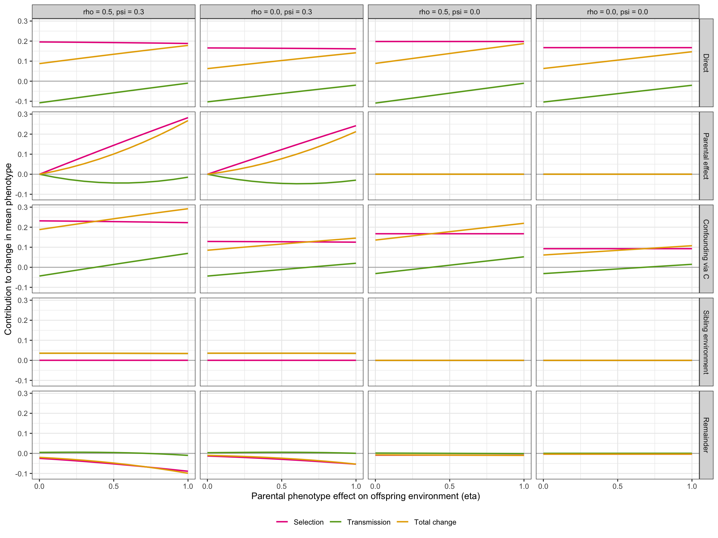
What this says about MR bias components
Every source of covariance between phenotype and parental contribution enters selection. How it splits between selection and transmission depends on its transmissibility, not on whether it would bias MR. In this model:
- The direct causal effect, which within-family MR targets, produces negative transmission in every setting. At the default settings and
eta = 0, its selection part is 0.196 and its transmission part −0.108, because less than half of the parental phenotypic variance reappears in offspring. This is the Price-equation form of the breeder’s equation: for this source, selection plus transmission equals the parent–offspring regression times the selection part. - The dynastic pathway (
eta) appears in both terms. Throughpsiit adds a selection part. Throughbeta_env * etait raises the transmissibility of every source that covaries with parental phenotype, which is why transmission rises withetain each row with a selection part. - Confounding through
C, the closest analogue here of population stratification, contributes negative transmission at lowetaand positive transmission at higheta, crossing zero where \(\tau_C = 1\). - The sibling environment has no selection part but adds about 0.035 to transmission whenever
psi > 0.
The MR bias components are therefore not confined to selection, and the MR residual is not the transmission term. MR splits the phenotype–fitness association into causal and non-causal parts; on the Price side, that split happens within selection. Each part then has a transmission counterpart, set by how faithfully it passes to offspring.
Two of the listed sources are not represented in the simulation. Pleiotropy, a genetic effect on fitness outside the phenotype, would enter as a term in the parental genetic score. Because the offspring score here is the parental score plus segregation noise, its transmissibility would be about 0.92 at eta = 0 under the default settings, so it would sit mostly in selection. That value favours genetic sources: in a diploid two-parent model, attributing offspring phenotypes to each parent separately would give per-parent genetic transmissibility of about one half, unless the mate’s genotype also covaries with the parent’s contribution. Assortative mating creates exactly that covariance, so it cannot be examined with one representative parent per family. The next section adds a second parent to examine both.
Two parents: assortative mating and pleiotropy
This section uses a separate, deliberately simpler model with two parents per family and a second trait \(Y\) that also affects fitness. It has no shared family environment, dynastic effect or stratification, so any difference between population and within-family MR comes from mate choice.
What pleiotropy changes
Pleiotropy, here an effect of the genetic score for \(Z\) on \(Y\), biases within-family MR as an estimate of the causal effect \(\theta\). It leaves the Price equation unchanged: the selection term is a phenotypic selection differential, and is indifferent to why phenotype and fitness covary. If \(Z\) has no causal effect but shares genes with a trait that does, \(Z\) still has nonzero selection and its mean still changes. Three quantities need to be kept apart:
| Question | Quantity | Is pleiotropy a bias? |
|---|---|---|
| Would changing \(Z\) change fitness? | \(\theta\), the target of within-family MR without pleiotropy | Yes |
| How much does the genetic component of mean \(Z\) change? | \(\alpha\operatorname{Cov}_N(w, G_Z)/\bar w\) (Robertson’s secondary theorem) | No, it is a correlated response |
| How is the phenotypic change split between selection and transmission? | Price terms | It changes the split |
With fitness \(W = 1 + \theta Z + \lambda Y + \dots\), \(Z = \alpha G_Z + \dots\) and \(Y = \alpha_Y G_Y + \kappa G_Z + \dots\), within-family MR targets \(\theta + \lambda\kappa/\alpha\). Under random mating, the genetic response is
\[ \frac{\alpha\operatorname{Cov}_N(w, G_Z)}{\bar w} = \left(\theta + \frac{\lambda\kappa}{\alpha}\right)\frac{\alpha^2\operatorname{Var}_N(G_Z)}{\bar w}, \]
which is within-family MR multiplied by the additive genetic variance of \(Z\). For predicting evolution, the pleiotropic part of the MR estimate is part of the answer, not a bias. The cost is that neither within-family MR nor the genetic response can separate causal from pleiotropic selection.
Model
Mothers and fathers are unrelated founders with independent, unit-variance genetic scores \(G_Z\) and \(G_Y\):
\[ Z = \alpha G_Z + \varepsilon_Z, \qquad Y = \alpha_Y G_Y + \kappa G_Z + \varepsilon_Y, \]
with \(\alpha = \alpha_Y = 0.5\) and noise SD 0.5, so the heritability of \(Z\) is 0.5. Mate choice is cross-trait: mothers ranked on a noisy score for \(Z\) are paired with fathers ranked on a noisy score for \(Y\), so that \(\operatorname{Cor}(Z_{\mathrm{mother}}, Y_{\mathrm{father}}) \approx r_{\mathrm{am}}\). Each couple has two offspring; each offspring genetic score is the mid-parent score plus segregation with variance 1/2. Offspring fitness, the MR outcome, is \(W_{\mathrm{off}} = 1 + \theta Z_{\mathrm{off}} + \lambda Y_{\mathrm{off}}\) plus noise, with \(\lambda = 0.5\).
Each couple is one Price ancestor: \(z_i\) is the mid-parent phenotype, and \(w_i = 1 + \theta\bar Z_i + \lambda\bar Y_i\) plus noise (floored at 0.05) is the couple’s shared reproductive contribution. Offspring descend from the couple, so the mate’s genes are part of the ancestor rather than a source of transmission.
Mate choice links the parents only through \(Z_{\mathrm{mother}}\) and \(Y_{\mathrm{father}}\). Offspring inherit a quarter of the resulting covariance between the mother’s \(G_Z\) and the father’s \(G_Y\). Within families, segregation of the two unlinked scores is independent, so within-family MR is unaffected, while population MR targets
\[ b_{\mathrm{population}} \longrightarrow \theta + \frac{\lambda\kappa}{\alpha} + \frac{\lambda\alpha_Y\operatorname{Cov}(G_{Z,\mathrm{off}}, G_{Y,\mathrm{off}})}{\alpha\operatorname{Var}(G_{Z,\mathrm{off}})}, \qquad \operatorname{Cov}(G_{Z,\mathrm{off}}, G_{Y,\mathrm{off}}) = \tfrac14\operatorname{Cov}(G_{Z,\mathrm{mother}}, G_{Y,\mathrm{father}}). \]
The last term is the assortative mating component of the MR residual.
simulate_couples <- function(
    n_couples = 20000, n_siblings = 2,
    theta = 0.20, lambda = 0.50, kappa = 0, r_am = 0,
    alpha = 0.50, alpha_y = 0.50, sigma = 0.50
) {
  stopifnot(
    length(r_am) == 1L, r_am >= 0, r_am <= 1,
    n_siblings >= 2, n_siblings == as.integer(n_siblings)
  )

  make_founders <- function(n) {
    G_Z <- rnorm(n)
    G_Y <- rnorm(n)
    data.frame(
      G_Z = G_Z, G_Y = G_Y,
      Z = alpha * G_Z + rnorm(n, sd = sigma),
      Y = alpha_y * G_Y + kappa * G_Z + rnorm(n, sd = sigma)
    )
  }
  mothers <- make_founders(n_couples)
  fathers <- make_founders(n_couples)

  # Each score correlates sqrt(r_am) with its trait; pairing by rank then gives
  # Cor(Z_mother, Y_father) close to r_am. With r_am = 0, mating is random but
  # the same random draws are used.
  mating_score <- function(x) {
    sqrt(r_am) * as.numeric(scale(x)) + sqrt(1 - r_am) * rnorm(length(x))
  }
  mothers <- mothers[order(mating_score(mothers$Z)), ]
  fathers <- fathers[order(mating_score(fathers$Y)), ]

  family_id <- rep(seq_len(n_couples), each = n_siblings)
  n_offspring <- length(family_id)
  G_Z_mid <- (mothers$G_Z + fathers$G_Z) / 2
  G_Y_mid <- (mothers$G_Y + fathers$G_Y) / 2
  # Segregation variance 1/2 keeps unit genetic variance under random mating.
  G_Z_off <- G_Z_mid[family_id] + rnorm(n_offspring, sd = sqrt(0.5))
  G_Y_off <- G_Y_mid[family_id] + rnorm(n_offspring, sd = sqrt(0.5))
  Z_off <- alpha * G_Z_off + rnorm(n_offspring, sd = sigma)
  Y_off <- alpha_y * G_Y_off + kappa * G_Z_off + rnorm(n_offspring, sd = sigma)
  W_off <- 1 + theta * Z_off + lambda * Y_off + rnorm(n_offspring, sd = 0.3)

  Z_mid <- (mothers$Z + fathers$Z) / 2
  Y_mid <- (mothers$Y + fathers$Y) / 2
  list(
    couples = data.frame(
      family_id = seq_len(n_couples),
      Z_mother = mothers$Z, Y_father = fathers$Y,
      G_Z_mid = G_Z_mid, Y_mid = Y_mid, Z_parent = Z_mid,
      W_parent = pmax(
        1 + theta * Z_mid + lambda * Y_mid + rnorm(n_couples, sd = 0.2), 0.05
      )
    ),
    offspring = data.frame(
      family_id = family_id, G_off = G_Z_off, Z_off = Z_off,
      Y_off = Y_off, W_off = W_off
    )
  )
}

couple_mr_targets <- function(
    theta, lambda, kappa, r_am, alpha = 0.50, alpha_y = 0.50, sigma = 0.50
) {
  var_z <- alpha^2 + sigma^2
  var_y <- alpha_y^2 + kappa^2 + sigma^2
  cov_mates <- r_am * sqrt(var_z * var_y)
  # Mother and father variables covary only through Z_mother and Y_father.
  cov_gz_gy_parents <- (alpha / var_z) * cov_mates * (alpha_y / var_y)
  cov_gz_gz_parents <- (alpha / var_z) * cov_mates * (kappa / var_y)
  var_gz_off <- 1 + cov_gz_gz_parents / 2
  cov_gz_gy_off <- cov_gz_gy_parents / 4

  within <- theta + lambda * kappa / alpha
  population <- within + lambda * alpha_y * cov_gz_gy_off / (alpha * var_gz_off)
  list(
    target_population = population,
    target_withinfamily = within,
    target_residual = population - within
  )
}
Price sources for couples
The couple’s contribution splits into the same kind of source terms as before:
| Source | Term in \(w\) |
|---|---|
| Direct | \(\theta\bar Z\) |
| Pleiotropy | \(\lambda\kappa\bar G_Z\) |
| Assortative mating | \(\lambda(\bar Y - \kappa\bar G_Z)\) |
| Remainder | Couple noise and the floor at 0.05 |
The assortative mating source is the part of the couple’s \(Y\) not caused by their \(G_Z\). Under random mating it is unrelated to the couple’s \(Z\); mate choice makes the father’s \(Y\) covary with the mother’s \(Z\). In the pleiotropy scenario, mate choice also links the mother’s \(Z\) to the father’s \(G_Z\) through his \(Y\), so part of the pleiotropy source depends on mate choice too.
# Split both Price terms by additive terms of the ancestors' contribution.
# The remainder makes both decompositions exact.
split_price <- function(terms, parents, offspring) {
  n <- nrow(parents)
  stopifnot(identical(parents$family_id, seq_len(n)))
  z <- parents$Z_parent
  dz <- family_means(offspring$Z_off, offspring$family_id, n) - z
  mean_w <- mean(parents$W_parent)
  terms[["Remainder"]] <- parents$W_parent - 1 - Reduce(`+`, terms)

  out <- data.frame(
    source = names(terms),
    selection = vapply(terms, cov_population, numeric(1), y = z) / mean_w,
    transmission = vapply(terms, cov_population, numeric(1), y = dz) / mean_w,
    row.names = NULL
  )
  is_remainder <- out$source == "Remainder"
  out$transmission[is_remainder] <- out$transmission[is_remainder] + mean(dz)
  out
}
The two scenarios have the same within-family MR target of 0.2: in the causal scenario through \(\theta = 0.2\), and in the pleiotropy scenario through \(\lambda\kappa/\alpha\) with \(\theta = 0\) and \(\kappa = 0.2\). Each sweeps the strength of mate choice from random mating to \(r_{\mathrm{am}} = 0.8\), resetting the seed for every run.
couple_scenarios <- data.frame(
  scenario = c("Causal", "Pleiotropy only"),
  theta = c(0.20, 0),
  kappa = c(0, 0.20),
  lambda = 0.50
)
r_am_values <- seq(0, 0.8, by = 0.1)

couple_runs <- do.call(c, lapply(seq_len(nrow(couple_scenarios)), function(s) {
  p <- couple_scenarios[s, ]
  lapply(r_am_values, function(r) {
    set.seed(4817)
    generations <- simulate_couples(
      theta = p$theta, lambda = p$lambda, kappa = p$kappa, r_am = r
    )
    couples <- generations$couples
    offspring <- generations$offspring
    mean_w <- mean(couples$W_parent)
    mr <- estimate_mr(offspring, nrow(couples))

    sources <- split_price(list(
      "Direct" = p$theta * couples$Z_parent,
      "Pleiotropy" = p$lambda * p$kappa * couples$G_Z_mid,
      "Assortative mating" = p$lambda * (couples$Y_mid - p$kappa * couples$G_Z_mid)
    ), couples, offspring)

    # alpha = 0.5 is the simulate_couples() default.
    summary <- data.frame(
      scenario = p$scenario, r_am = r,
      r_mates = cor(couples$Z_mother, couples$Y_father),
      mr,
      couple_mr_targets(p$theta, p$lambda, p$kappa, r),
      estimate_price(couples, assign_offspring_weights(couples, offspring)),
      genetic_response =
        0.5 * cov_population(couples$W_parent, couples$G_Z_mid) / mean_w,
      mr_withinfamily_va = mr$b_withinfamily * 0.5^2 *
        cov_population(couples$G_Z_mid, couples$G_Z_mid) / mean_w
    )
    list(summary = summary, sources = cbind(scenario = p$scenario, r_am = r, sources))
  })
}))
couple_results <- do.call(rbind, lapply(couple_runs, `[[`, "summary"))
couple_sources <- do.call(rbind, lapply(couple_runs, `[[`, "sources"))

stopifnot(all(abs(couple_results$price_error) < 1e-12))
local({
  totals <- aggregate(
    cbind(selection, transmission) ~ scenario + r_am, couple_sources, sum
  )
  matched <- merge(totals, couple_results[, c(
    "scenario", "r_am", "price_selection", "price_transmission"
  )])
  stopifnot(
    nrow(matched) == nrow(couple_results),
    all(abs(matched$selection - matched$price_selection) < 1e-10),
    all(abs(matched$transmission - matched$price_transmission) < 1e-10)
  )
})

knitr::kable(
  couple_results[couple_results$r_am %in% range(r_am_values), c(
    "scenario", "r_am", "r_mates", "b_withinfamily", "b_population",
    "price_selection", "price_transmission", "delta_z",
    "genetic_response", "mr_withinfamily_va"
  )],
  digits = 3, row.names = FALSE,
  col.names = c(
    "Scenario", "r_am", "Realised Cor(Z_m, Y_f)", "Within-family MR",
    "Population MR", "Selection", "Transmission", "Total change",
    "Genetic response", "Within-family MR × V_A"
  )
)| Scenario | r_am | Realised Cor(Z_m, Y_f) | Within-family MR | Population MR | Selection | Transmission | Total change | Genetic response | Within-family MR × V_A |
|---|---|---|---|---|---|---|---|---|---|
| Causal | 0.0 | -0.005 | 0.207 | 0.203 | 0.047 | -0.022 | 0.026 | 0.024 | 0.026 |
| Causal | 0.8 | 0.799 | 0.207 | 0.257 | 0.099 | -0.047 | 0.052 | 0.050 | 0.026 |
| Pleiotropy only | 0.0 | -0.006 | 0.207 | 0.205 | 0.022 | 0.004 | 0.026 | 0.024 | 0.026 |
| Pleiotropy only | 0.8 | 0.800 | 0.207 | 0.252 | 0.078 | -0.025 | 0.054 | 0.053 | 0.030 |
plot_couple_mr <- function(couple_results) {
  series <- c("Population", "Within-family", "Residual")
  types <- c("Simulated", "Large-sample target")
  n <- nrow(couple_results)
  long <- data.frame(
    scenario = couple_results$scenario, r_am = couple_results$r_am,
    series = factor(rep(rep(series, each = n), 2), levels = series),
    type = factor(rep(types, each = 3 * n), levels = types),
    value = with(couple_results, c(
      b_population, b_withinfamily, b_residual,
      target_population, target_withinfamily, target_residual
    ))
  )

  ggplot(long, aes(r_am, value, colour = series, linetype = type)) +
    geom_hline(yintercept = 0.2, colour = "grey70") +
    geom_line(linewidth = 0.8) +
    # Dark2 colours 1-3, matching the MR lines in fig-mr-price-comparison.
    scale_colour_manual(values = setNames(c("#1B9E77", "#D95F02", "#7570B3"), series)) +
    scale_linetype_manual(values = setNames(c("solid", "dotted"), types)) +
    facet_wrap(~ scenario) +
    labs(
      x = "Strength of cross-trait assortative mating (r_am)",
      y = "MR estimate", colour = NULL, linetype = NULL
    ) +
    theme_bw() +
    theme(legend.position = "bottom")
}
plot_couple_mr(couple_results)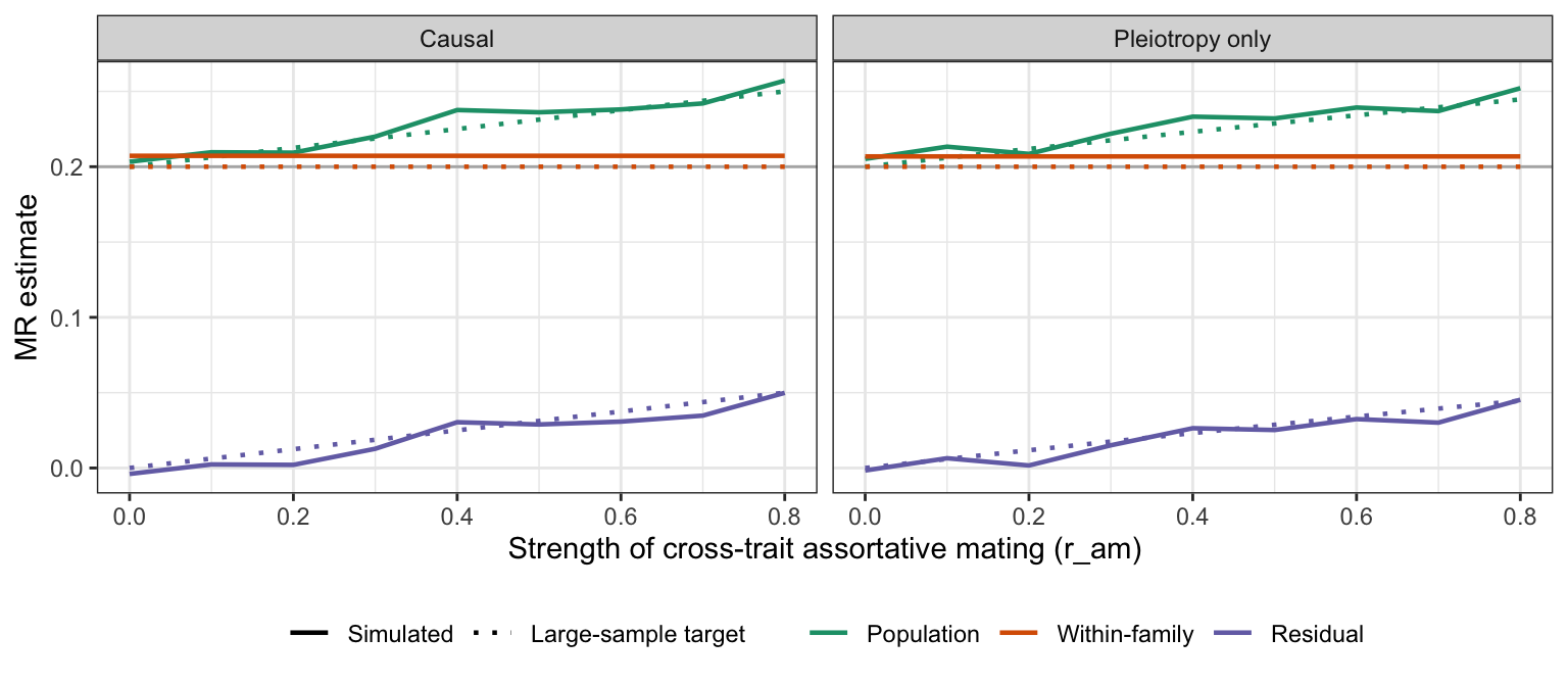
plot_couple_sources <- function(couple_results, couple_sources) {
  all_sources <- data.frame(
    scenario = couple_results$scenario, r_am = couple_results$r_am,
    source = "All sources",
    selection = couple_results$price_selection,
    transmission = couple_results$price_transmission
  )
  x <- rbind(all_sources, couple_sources)
  x$source <- factor(x$source, levels = unique(x$source))
  terms <- c("Selection", "Transmission", "Total change")
  long <- data.frame(
    scenario = x$scenario, source = x$source, r_am = x$r_am,
    term = factor(rep(terms, each = nrow(x)), levels = terms),
    value = c(x$selection, x$transmission, x$selection + x$transmission)
  )

  ggplot(long, aes(r_am, value, colour = term)) +
    geom_hline(yintercept = 0, colour = "grey70") +
    geom_line(linewidth = 0.8) +
    scale_colour_manual(values = setNames(c("#E7298A", "#66A61E", "#E6AB02"), terms)) +
    facet_grid(source ~ scenario) +
    labs(
      x = "Strength of cross-trait assortative mating (r_am)",
      y = "Contribution to change in mean phenotype", colour = NULL
    ) +
    theme_bw() +
    theme(legend.position = "bottom")
}
plot_couple_sources(couple_results, couple_sources)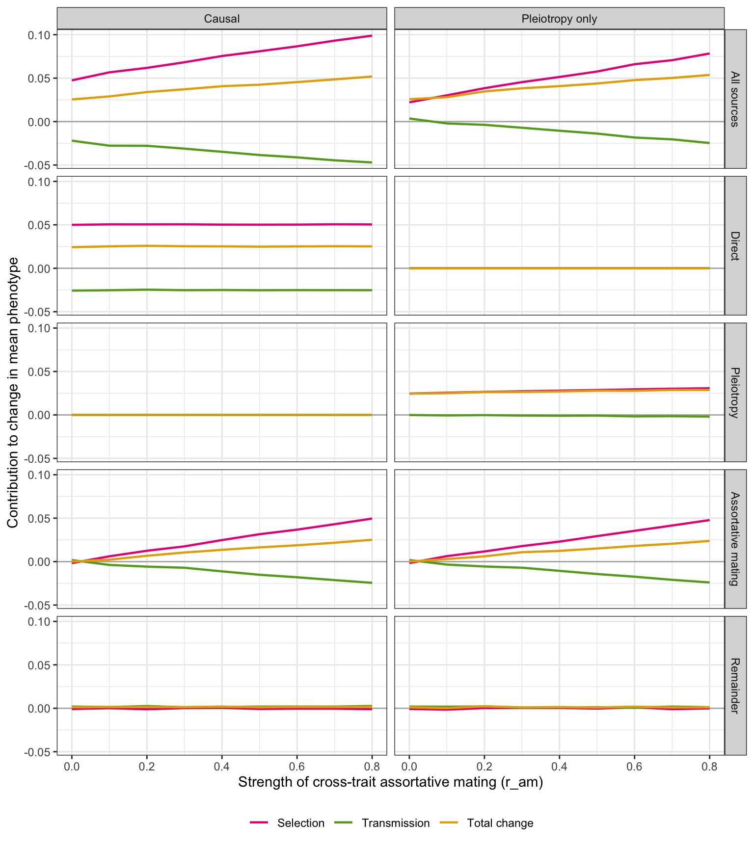
What the two-parent model shows
MR cannot tell the two scenarios apart (Figure 4). Within-family MR is about 0.21 in both, against a target of 0.2; the runs share random draws, so the sampling error is common to all of them. Population MR rises with mate choice in both, by about 0.05 at \(r_{\mathrm{am}} = 0.8\). That rise is the assortative mating component of the residual, and it matches the large-sample target.
The Price terms do differ (Figure 5). Under random mating, both scenarios give the same total change (0.026) and genetic response (0.024), but split differently:
- In the causal scenario, fitness depends on all of \(Z\), including its non-heritable part. Selection is 0.047 and transmission −0.022, so the direct source’s transmissibility is about 0.5, the heritability of \(Z\).
- In the pleiotropy scenario, fitness depends on genes shared with \(Z\), and the change in genetic value is passed on fully. Selection is 0.022 and transmission about zero, so the source’s transmissibility is about 1.
Assortative mating adds to both Price terms in both scenarios. At \(r_{\mathrm{am}} = 0.8\), the assortative mating source has selection 0.05 and transmission −0.024. Transmissibility is again about 0.5, because mate choice acts on the mother’s phenotype, of which offspring inherit only the genetic part. If mates sorted on genotype instead, more of this selection would be transmitted.
The genetic response tracks the total change in both scenarios, but within-family MR × \(V_A\) stays near 0.026–0.030 as mate choice strengthens. The extra response under assortative mating runs through the mate: mothers with high \(Z\) have partners with high \(Y\), and so a higher couple contribution. Within-family MR excludes this pathway by design. Within-family MR × \(V_A\) therefore matches the genetic response only under random mating, consistent with the derivation above.
So what are we interpreting? Within-family MR estimates \(\theta\) only in the absence of pleiotropy. Read instead as a genetic regression scaled to \(Z\), it gives the part of the genetic response that runs through each individual’s own genes, whether causally through \(Z\) or through pleiotropy. The Price selection term is a phenotypic selection differential. How it splits between selection and transmission depends on whether selection acts on all phenotypic variation or only on its transmitted part, which is information MR alone does not carry. Other sources with transmissibility below one, such as the shared environment in the one-parent model, would blur this contrast. None of the MR bias components here—pleiotropy, assortative mating, and the dynastic and stratification-like paths in the one-parent model—maps onto selection alone.
Two simplifications matter. The founders have no history of assortative mating, so the model shows a single generation of mate choice rather than the accumulated genetic correlation at equilibrium. Mate choice is also one-directional, pairing mothers’ \(Z\) with fathers’ \(Y\). Symmetric cross-trait mate choice would be expected to strengthen both the MR residual and the Price assortative mating source.