Quantile regression GWAS

Author

Gibran Hemani

Published

July 9, 2026

Background

rif_quantile <- function(Y, tau = 0.5, na.rm = TRUE, bw = "nrd0") {
  stopifnot(is.numeric(Y))
  stopifnot(length(tau) == 1, tau > 0, tau < 1)
  
  # Keep track of missingness
  out <- rep(NA_real_, length(Y))
  ok <- !is.na(Y)
  Y0 <- Y[ok]
  
  # Estimate empirical quantile
  q_tau <- as.numeric(quantile(Y0, probs = tau, na.rm = na.rm, type = 7))
  
  # Estimate density at the quantile
  dens <- density(Y0, na.rm = na.rm, bw = bw)
  f_q <- approx(dens$x, dens$y, xout = q_tau, rule = 2)$y
  
  # RIF for quantile
  out[ok] <- q_tau + (tau - as.numeric(Y0 <= q_tau)) / f_q
  
  attr(out, "tau") <- tau
  attr(out, "q_tau") <- q_tau
  attr(out, "f_q") <- f_q
  
  return(out)
}

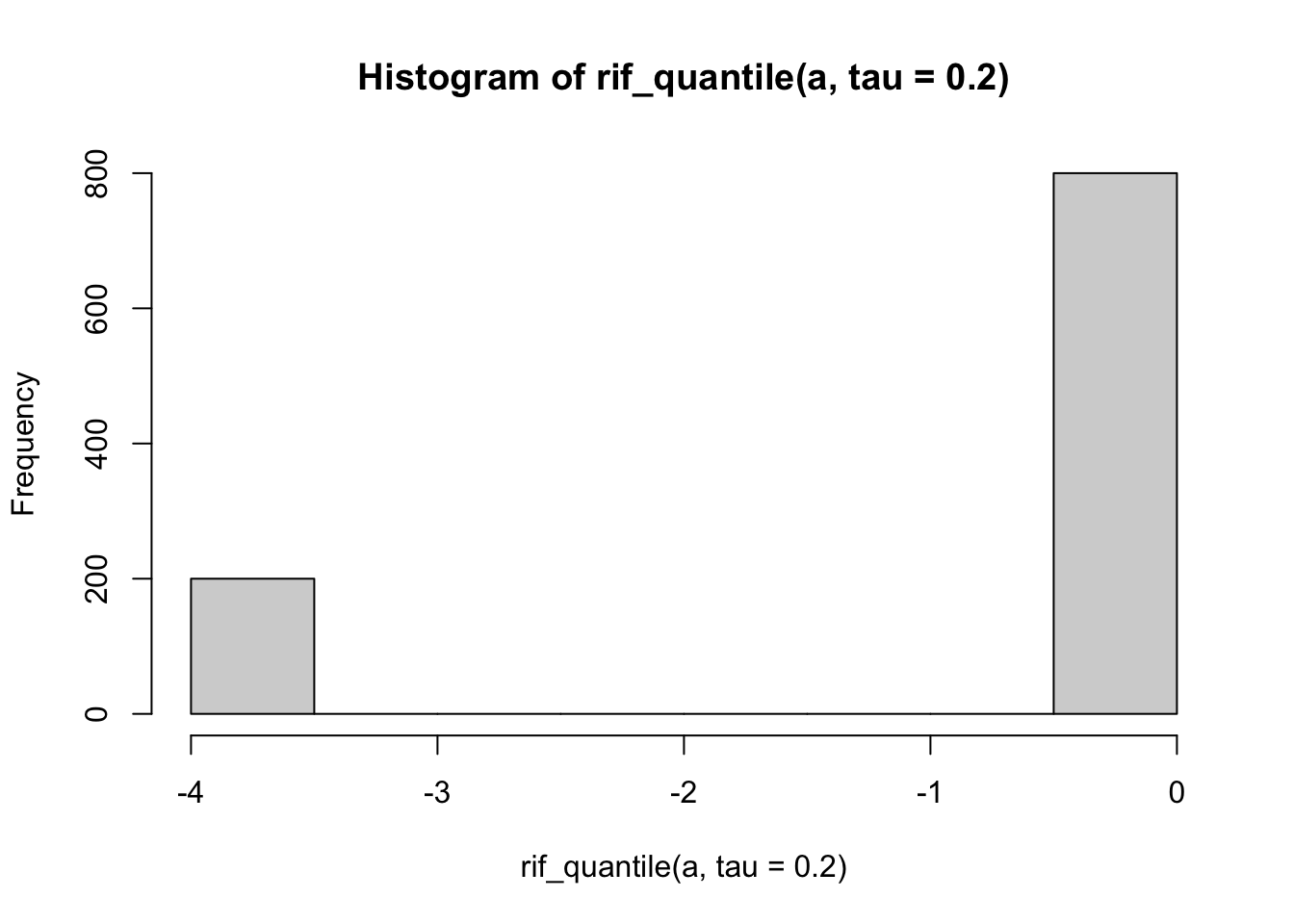
a <- rnorm(1000)
hist(rif_quantile(a, tau = 0.2))

set.seed(1)

set.seed(123)

# -----------------------------
# 1. Simulate data
# -----------------------------

n <- 20000

sex <- rbinom(n, 1, 0.5)  # 0 = female, 1 = male
G   <- rbinom(n, 2, 0.3)  # SNP dosage: 0, 1, 2

# Parameters
mu_female <- 0
mu_male   <- 3
sd_y      <- 1

beta_female <- 0
beta_male   <- 0.5

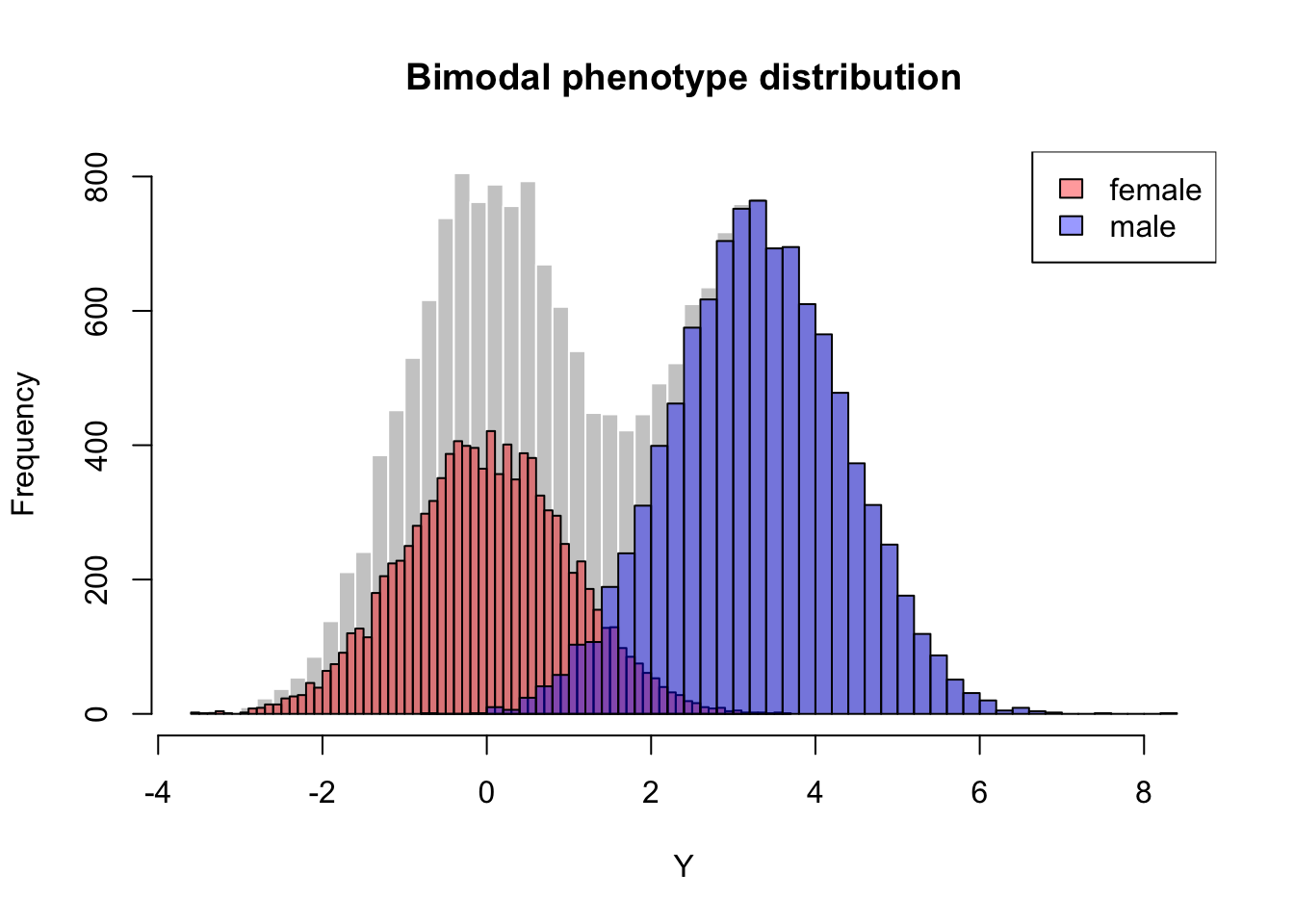
# Phenotype: bimodal due to sex, SNP effect only in males
Y <- mu_female * (1 - sex) +
     mu_male   * sex +
     beta_female * G * (1 - sex) +
     beta_male   * G * sex +
     rnorm(n, mean = 0, sd = sd_y)

dat <- data.frame(Y, G, sex = factor(sex, labels = c("female", "male")))

hist(dat$Y, breaks = 80, col = "grey80", border = "white",
     main = "Bimodal phenotype distribution",
     xlab = "Y")

hist(dat$Y[dat$sex == "female"], breaks = 60, col = rgb(1, 0, 0, 0.4),
     add = TRUE)
hist(dat$Y[dat$sex == "male"], breaks = 60, col = rgb(0, 0, 1, 0.4),
     add = TRUE)

legend("topright",
       legend = c("female", "male"),
       fill = c(rgb(1, 0, 0, 0.4), rgb(0, 0, 1, 0.4)))
summary(lm(Y ~ G * sex, data = dat))

Call:
lm(formula = Y ~ G * sex, data = dat)

Residuals:
    Min      1Q  Median      3Q     Max 
-4.1194 -0.6771  0.0012  0.6810  4.3375 

Coefficients:
            Estimate Std. Error t value Pr(>|t|)    
(Intercept)  0.00616    0.01337   0.461    0.645    
G           -0.01821    0.01513  -1.204    0.229    
sexmale      2.98900    0.01916 156.033   <2e-16 ***
G:sexmale    0.51331    0.02178  23.571   <2e-16 ***
---
Signif. codes:  0 '***' 0.001 '**' 0.01 '*' 0.05 '.' 0.1 ' ' 1

Residual standard error: 0.9998 on 19996 degrees of freedom
Multiple R-squared:  0.7343,    Adjusted R-squared:  0.7342 
F-statistic: 1.842e+04 on 3 and 19996 DF,  p-value: < 2.2e-16
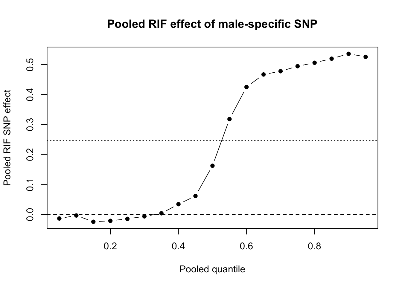
taus <- seq(0.05, 0.95, by = 0.05)

rif_results_pooled <- lapply(taus, function(tau) {
  dat$rif <- rif_quantile(dat$Y, tau = tau)
  fit <- lm(rif ~ G, data = dat)
  
  data.frame(
    tau = tau,
    q_tau = attr(dat$rif, "q_tau"),
    f_q = attr(dat$rif, "f_q"),
    beta_G = coef(fit)["G"],
    se_G = summary(fit)$coefficients["G", "Std. Error"]
  )
})

rif_results_pooled <- do.call(rbind, rif_results_pooled)
rif_results_pooled
     tau       q_tau        f_q       beta_G       se_G
G   0.05 -1.29106323 0.09192478 -0.013724177 0.02580581
G1  0.10 -0.86285437 0.13796583 -0.003692038 0.02366769
G2  0.15 -0.54017970 0.17340861 -0.024558255 0.02241185
G3  0.20 -0.28591407 0.19094958 -0.021464792 0.02280017
G4  0.25 -0.02619083 0.19431518 -0.014783399 0.02425472
G5  0.30  0.23113297 0.19157219 -0.006740053 0.02603651
G6  0.35  0.49010154 0.18344252  0.003519377 0.02830068
G7  0.40  0.76502260 0.16359150  0.033888660 0.03259414
G8  0.45  1.11317175 0.13345351  0.061380649 0.04057319
G9  0.50  1.53776264 0.11200616  0.162343825 0.04857505
G10 0.55  1.99390584 0.11881333  0.317900016 0.04551975
G11 0.60  2.39109314 0.14166673  0.424948284 0.03751938
G12 0.65  2.71746243 0.16356664  0.466800355 0.03156755
G13 0.70  3.00329291 0.17934265  0.477489604 0.02760629
G14 0.75  3.26424219 0.18340877  0.494256649 0.02545847
G15 0.80  3.54147292 0.17619319  0.505992850 0.02444983
G16 0.85  3.82865465 0.15890387  0.519560877 0.02418082
G17 0.90  4.16996746 0.13050066  0.535832867 0.02473303
G18 0.95  4.63583771 0.08442225  0.525700141 0.02785236
plot(rif_results_pooled$tau,
     rif_results_pooled$beta_G,
     type = "b",
     pch = 16,
     xlab = "Pooled quantile",
     ylab = "Pooled RIF SNP effect",
     main = "Pooled RIF effect of male-specific SNP")
abline(h = 0, lty = 2)
abline(h = beta_male * mean(sex), lty = 3)

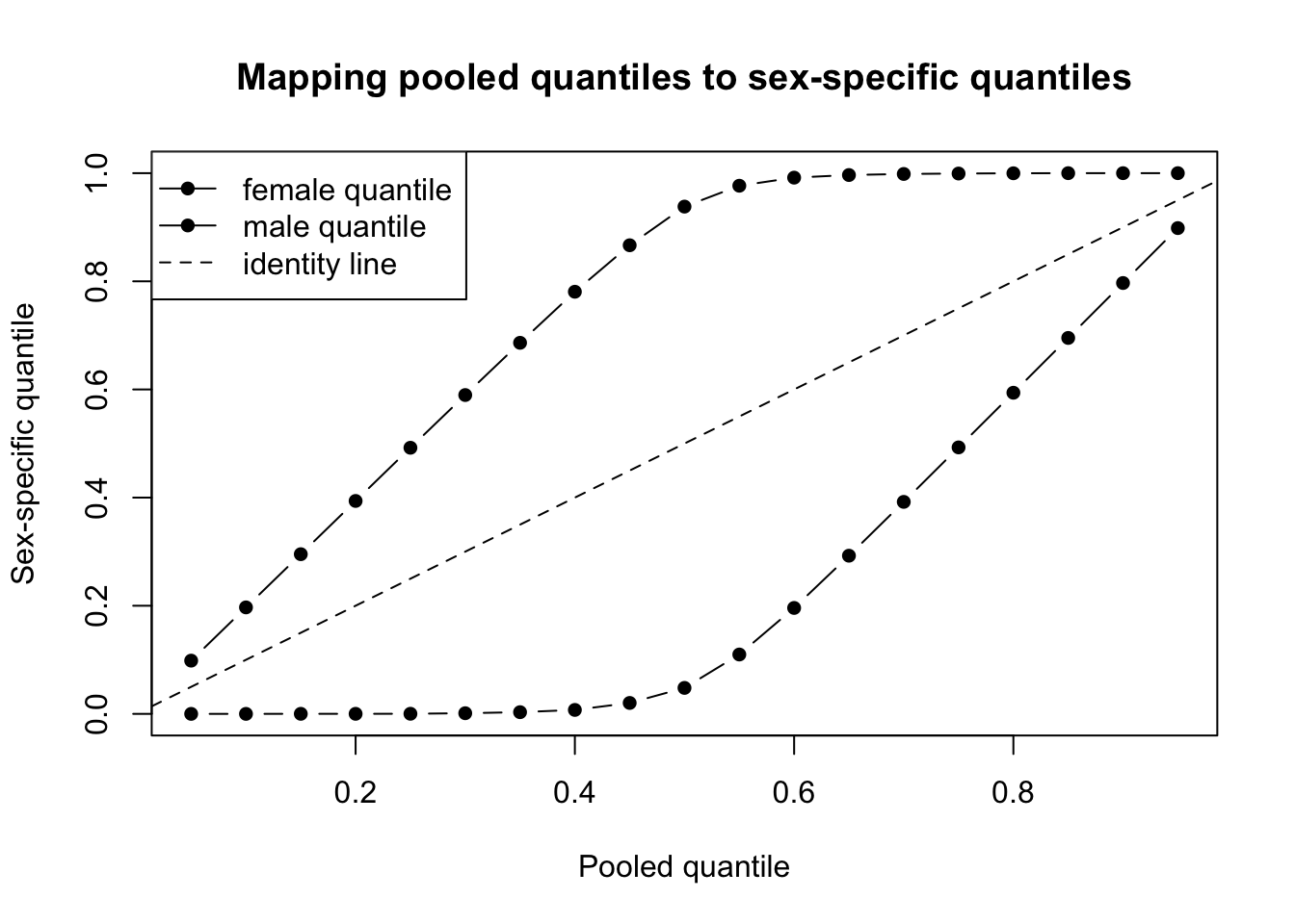
quantile_map <- lapply(taus, function(tau) {
  q_tau <- as.numeric(quantile(dat$Y, tau))
  
  data.frame(
    tau_pooled = tau,
    q_tau = q_tau,
    female_quantile = mean(dat$Y[dat$sex == "female"] <= q_tau),
    male_quantile = mean(dat$Y[dat$sex == "male"] <= q_tau)
  )
})

quantile_map <- do.call(rbind, quantile_map)
quantile_map
   tau_pooled       q_tau female_quantile male_quantile
1        0.05 -1.29106323      0.09847366  0.0000000000
2        0.10 -0.86285437      0.19694732  0.0000000000
3        0.15 -0.54017970      0.29532250  0.0001015744
4        0.20 -0.28591407      0.39379616  0.0001015744
5        0.25 -0.02619083      0.49217134  0.0002031488
6        0.30  0.23113297      0.58966027  0.0012188928
7        0.35  0.49010154      0.68626292  0.0031488065
8        0.40  0.76502260      0.78069916  0.0073133570
9        0.45  1.11317175      0.86666667  0.0202133062
10       0.50  1.53776264      0.93815854  0.0480446927
11       0.55  1.99390584      0.97676022  0.1098019299
12       0.60  2.39109314      0.99172821  0.1959370239
13       0.65  2.71746243      0.99655342  0.2925342814
14       0.70  3.00329291      0.99852290  0.3920771965
15       0.75  3.26424219      0.99931068  0.4928390046
16       0.80  3.54147292      0.99980305  0.5939055358
17       0.85  3.82865465      1.00000000  0.6952767902
18       0.90  4.16996746      1.00000000  0.7968511935
19       0.95  4.63583771      1.00000000  0.8984255967
plot(quantile_map$tau_pooled,
     quantile_map$female_quantile,
     type = "b",
     pch = 16,
     ylim = c(0, 1),
     xlab = "Pooled quantile",
     ylab = "Sex-specific quantile",
     main = "Mapping pooled quantiles to sex-specific quantiles")

lines(quantile_map$tau_pooled,
      quantile_map$male_quantile,
      type = "b",
      pch = 16)

abline(0, 1, lty = 2)

legend("topleft",
       legend = c("female quantile", "male quantile", "identity line"),
       lty = c(1, 1, 2),
       pch = c(16, 16, NA))


sessionInfo()
R version 4.6.0 (2026-04-24)
Platform: aarch64-apple-darwin23
Running under: macOS Sequoia 15.2

Matrix products: default
BLAS:   /Library/Frameworks/R.framework/Versions/4.6/Resources/lib/libRblas.0.dylib 
LAPACK: /Library/Frameworks/R.framework/Versions/4.6/Resources/lib/libRlapack.dylib;  LAPACK version 3.12.1

locale:
[1] en_US.UTF-8/en_US.UTF-8/en_US.UTF-8/C/en_US.UTF-8/en_US.UTF-8

time zone: Europe/London
tzcode source: internal

attached base packages:
[1] stats     graphics  grDevices utils     datasets  methods   base     

loaded via a namespace (and not attached):
 [1] htmlwidgets_1.6.4 compiler_4.6.0    fastmap_1.2.0     cli_3.6.6        
 [5] tools_4.6.0       htmltools_0.5.9   otel_0.2.0        yaml_2.3.12      
 [9] rmarkdown_2.31    knitr_1.51        jsonlite_2.0.0    xfun_0.57        
[13] digest_0.6.39     rlang_1.2.0       evaluate_1.0.5