Conditioning on the exposure

Author

Gibran Hemani

Published

June 22, 2026

Background

A tempting solution to the pleiotropy problem in MR is to check if the instrument associates with the outcome conditioning on the exposure. Under the assumption that X and Y are confounded, this opens a collider path to Y. Meaning that by default we expect the instrument to associate with the outcome conditional on the exposure. This is a problem because it means that we cannot use this as a test for pleiotropy.

This simulation examines how sensitive the association between the instrument and outcome is to conditioning on the exposure. The simulation is based on a simple model where X and Y are confounded by U, and the instrument Z is associated with X but not Y. i.e. There is no pleiotropy - so any association between Z and Y conditional on X is due to the collider path, and will lead to erroneously disgarding the instrument.

Simulation

library(tidyverse)
── Attaching core tidyverse packages ──────────────────────── tidyverse 2.0.0 ──
✔ dplyr     1.2.1     ✔ readr     2.2.0
✔ forcats   1.0.1     ✔ stringr   1.6.0
✔ ggplot2   4.0.3     ✔ tibble    3.3.1
✔ lubridate 1.9.5     ✔ tidyr     1.3.2
✔ purrr     1.2.2     
── Conflicts ────────────────────────────────────────── tidyverse_conflicts() ──
✖ dplyr::filter() masks stats::filter()
✖ dplyr::lag()    masks stats::lag()
ℹ Use the conflicted package (<http://conflicted.r-lib.org/>) to force all conflicts to become errors
library(furrr)
Loading required package: future
library(here)
here() starts at /Users/gh13047/repo/lab-book
fast_assoc <- function(y, x)
{
    index <- is.finite(y) & is.finite(x)
    n <- sum(index)
    y <- y[index]
    x <- x[index]
    vx <- var(x)
    bhat <- stats::cov(y, x) / vx
    ahat <- mean(y) - bhat * mean(x)
    # fitted <- ahat + x * bhat
    # residuals <- y - fitted
    # SSR <- sum((residuals - mean(residuals))^2)
    # SSF <- sum((fitted - mean(fitted))^2)

    rsq <- (bhat * vx)^2 / (vx * var(y))
    fval <- rsq * (n-2) / (1-rsq)
    tval <- sqrt(fval)
    se <- abs(bhat / tval)

    # Fval <- (SSF) / (SSR/(n-2))
    # pval <- pf(Fval, 1, n-2, lowe=F)
    p <- stats::pf(fval, 1, n-2, lower.tail=FALSE)
    return(list(
        ahat=ahat, bhat=bhat, se=se, fval=fval, pval=p, n=n
    ))
}

make_dat <- function(n=1000, bxy=0.5, bxz=0.5, byu=0.5, bxu=0.5)
{
    u <- rnorm(n)
    z <- rnorm(n)
    x <- bxz * z + bxu * u + rnorm(n)
    y <- bxy * x + byu * u + rnorm(n)

    dat <- data.frame(u=u, z=z, x=x, y=y)
    return(dat)
}

estimation <- function(dat)
{
    # estimate the association between Z and Y
    res1 <- fast_assoc(dat$y, dat$z)
    res2 <- fast_assoc(dat$x, dat$z)

    # estimate the association between Z and Y conditional on X
    res2 <- fast_assoc(lm(y ~ x, data=dat)$residuals, dat$z)

    tibble(
        rsq_xy=cor(dat$x, dat$y)^2,
        rsq_xz=cor(dat$x, dat$z)^2,
        rsq_yz=cor(dat$y, dat$z)^2,
        rsq_yu=cor(dat$y, dat$u)^2,
        rsq_xu=cor(dat$x, dat$u)^2,
        pval_xz=res1$pval,
        fval=res1$fval,
        pval=res1$pval,
        pval_cond=res2$pval
    )
}

sim <- function(n=1000, bxy=0.5, bxz=0.5, byu=0.5, bxu=0.5)
{
    dat <- make_dat(n=n, bxy=bxy, bxz=bxz, byu=byu, bxu=bxu)
    res <- estimation(dat)
    return(res)
}

sim(n=100000, bxy=0.5, bxz=0.2, byu=0.5, bxu=0.5)
# A tibble: 1 × 9
  rsq_xy rsq_xz  rsq_yz rsq_yu rsq_xu   pval_xz  fval      pval pval_cond
   <dbl>  <dbl>   <dbl>  <dbl>  <dbl>     <dbl> <dbl>     <dbl>     <dbl>
1  0.337 0.0316 0.00595  0.307  0.191 8.95e-132  598. 8.95e-132  4.04e-24
params <- expand.grid(
    n=c(100000),
    bxy=c(0),
    bxz=seq(0, 0.04, by=0.01),
    byu=seq(0, 1, by=0.2),
    bxu=seq(0, 1, by=0.2),
    simrep=1:100
)

dim(params)
plan(multisession, workers=8)
results <- future_pmap(
    params,
    function(n, bxy, bxz, byu, bxu, simrep) {
        sim(n=n, bxy=bxy, bxz=bxz, byu=byu, bxu=bxu)
    }, .options = furrr_options(seed = TRUE), .progress = TRUE
) %>% bind_rows()

# results <- params[1:100,] |>
#   rowwise() |>
#   mutate(sim = list(sim(n=n, bxy=bxy, bxz=bxz, byu=byu, bxu=bxu))) |>
#   unnest(sim)

results <- bind_cols(results, params)
saveRDS(results, here("posts/2026-06-22-conditioning-ont-he-exposure", "results.rds"))
results <- readRDS(here("posts/2026-06-22-conditioning-ont-he-exposure", "results.rds"))
sumres <- results %>%
    group_by(bxu) %>% mutate(rsq_xu = mean(rsq_xu) %>% round(2)) %>%
    group_by(byu) %>% mutate(rsq_yu = mean(rsq_yu) %>% round(2)) %>%
    ungroup() %>%
    group_by(bxz, rsq_yu, rsq_xu) %>%
    summarise(
        mean_rsq_xz = mean(rsq_xz),
        mean_pval_xz = mean(-log10(pval_xz)),
        mean_pval_cond = mean(pval_cond),
        pow_cond = mean(pval_cond < 0.05)
    ) %>%
    ungroup()
`summarise()` has regrouped the output.
ℹ Summaries were computed grouped by bxz, rsq_yu, and rsq_xu.
ℹ Output is grouped by bxz and rsq_yu.
ℹ Use `summarise(.groups = "drop_last")` to silence this message.
ℹ Use `summarise(.by = c(bxz, rsq_yu, rsq_xu))` for per-operation grouping
  (`?dplyr::dplyr_by`) instead.
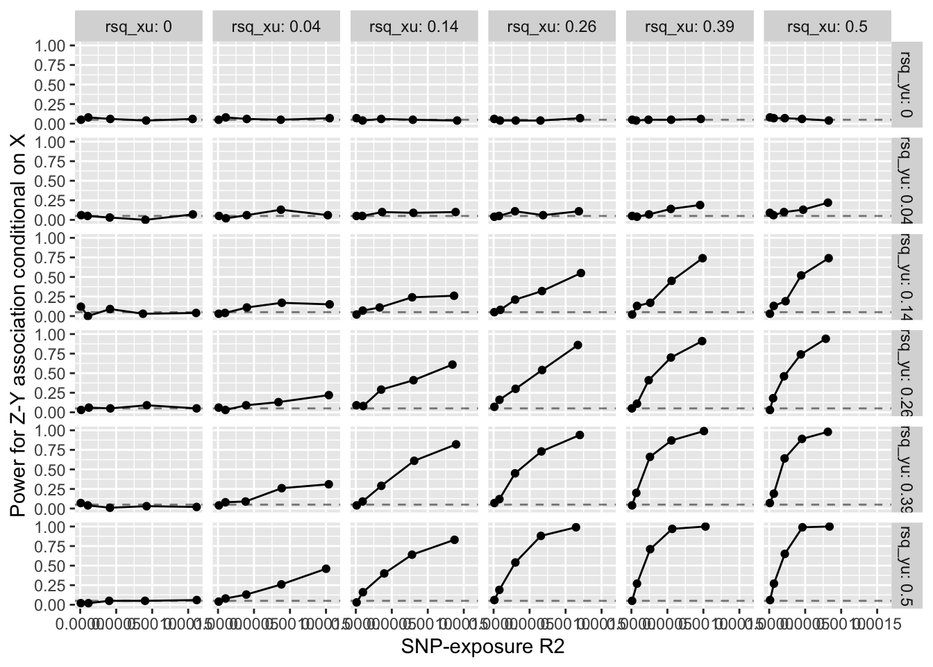
ggplot(sumres, aes(x=mean_rsq_xz, y=pow_cond)) +
  geom_point() +
  geom_line() +
  labs(x="SNP-exposure R2", y="Power for Z-Y association conditional on X") +
  geom_hline(yintercept=0.05, linetype="dashed", alpha=0.5) +
  facet_grid(rsq_yu ~ rsq_xu, labeller = label_both)

What if we have lots of instruments?

Is there a constant collider bias, meaning that all residual effects of instrument on Y will be the same + horizontal pleiotropy?

gwas <- function(z, y) {
    for(i in 1:ncol(z)) {
        Z <- as.numeric(unlist(z[,i]))
        res <- fast_assoc(y, Z)
        if (i == 1) {
            out <- as_tibble(res) %>% mutate(snp=i)
        } else {
            out <- bind_rows(out, as_tibble(res) %>% mutate(snp=i))
        }
    }
    return(out)
}

make_dat <- function(params)
{
    nsnp <- params$nsnp
    prop_pleio <- params$prop_pleio
    n <- params$n
    bxy <- params$bxy
    bxz <- params$bxz
    byu <- params$byu
    bxu <- params$bxu
    bzx <- params$bzx
    bzy <- params$bzy

    u <- rnorm(n)
    z <- matrix(rnorm(n * nsnp), nrow=n, ncol=nsnp)
    zx <- z %*% bzx %>% drop
    zy <- z %*% bzy %>% drop
    x <- bxz * zx + bxu * u + rnorm(n)
    y <- bxy * x + zy + byu * u + rnorm(n)

    z <- as.data.frame(z)
    names(z) <- paste0("z", 1:nsnp)

    dat <- tibble(u=u, x=x, y=y) %>% bind_cols(z)
    return(dat)
}


make_params <- function(nsnp=100, prop_pleio=0.5, n=1000, bxy=0.5, bxz=0.5, byu=0.5, bxu=0.5) {
    bzx <- rnorm(nsnp, 0, 0.1)
    bzy <- rnorm(nsnp, 0, 0.1) * sample(c(0,1), nsnp, replace=TRUE, prob=c(1-prop_pleio, prop_pleio))

    list(
        nsnp=nsnp,
        prop_pleio=prop_pleio,
        n=n,
        bxy=bxy,
        bxz=bxz,
        byu=byu,
        bxu=bxu,
        bzx=bzx,
        bzy=bzy
    )
}

estimation <- function(dat)
{
    # estimate the association between Z and Y
    # res1 <- gwas(dat[,4:ncol(dat)], dat$y)
    # res2 <- gwas(dat[,4:ncol(dat)], dat$x)

    # estimate the association between Z and Y conditional on X
    res3 <- gwas(dat[,4:ncol(dat)], lm(y ~ x, data=dat)$residuals)
    return(res3)
    bind_rows(
        res1 %>% mutate(type="Z-Y"),
        res2 %>% mutate(type="Z-X"),
        res3 %>% mutate(type="Z-Y|X")
    )
}
p <- make_params(n=100000)
dat <- make_dat(p)
res <- estimation(dat)
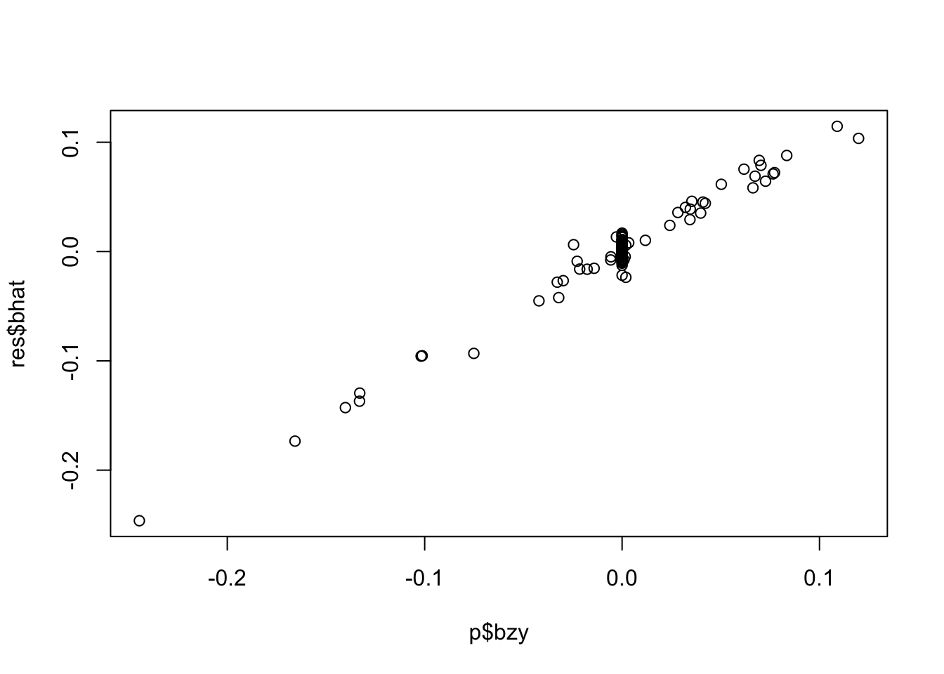
plot(res$bhat ~ p$bzy)

p <- make_params(n=100000, byu = 1, bxu = 1, bxy=0.5, prop_pleio = 0.5)
dat <- make_dat(p)
res <- estimation(dat)
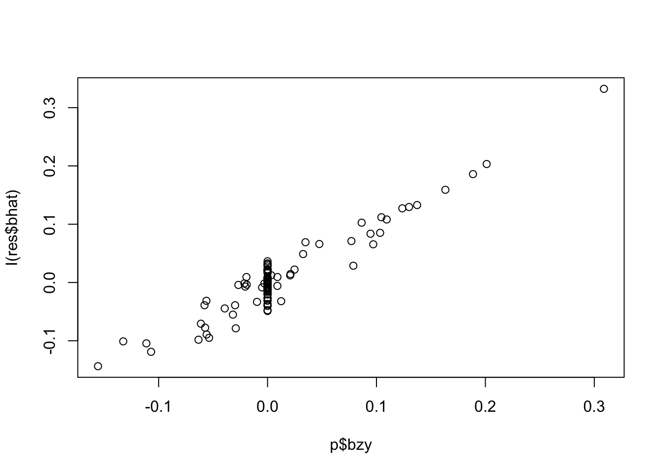
plot(I(res$bhat) ~ p$bzy)

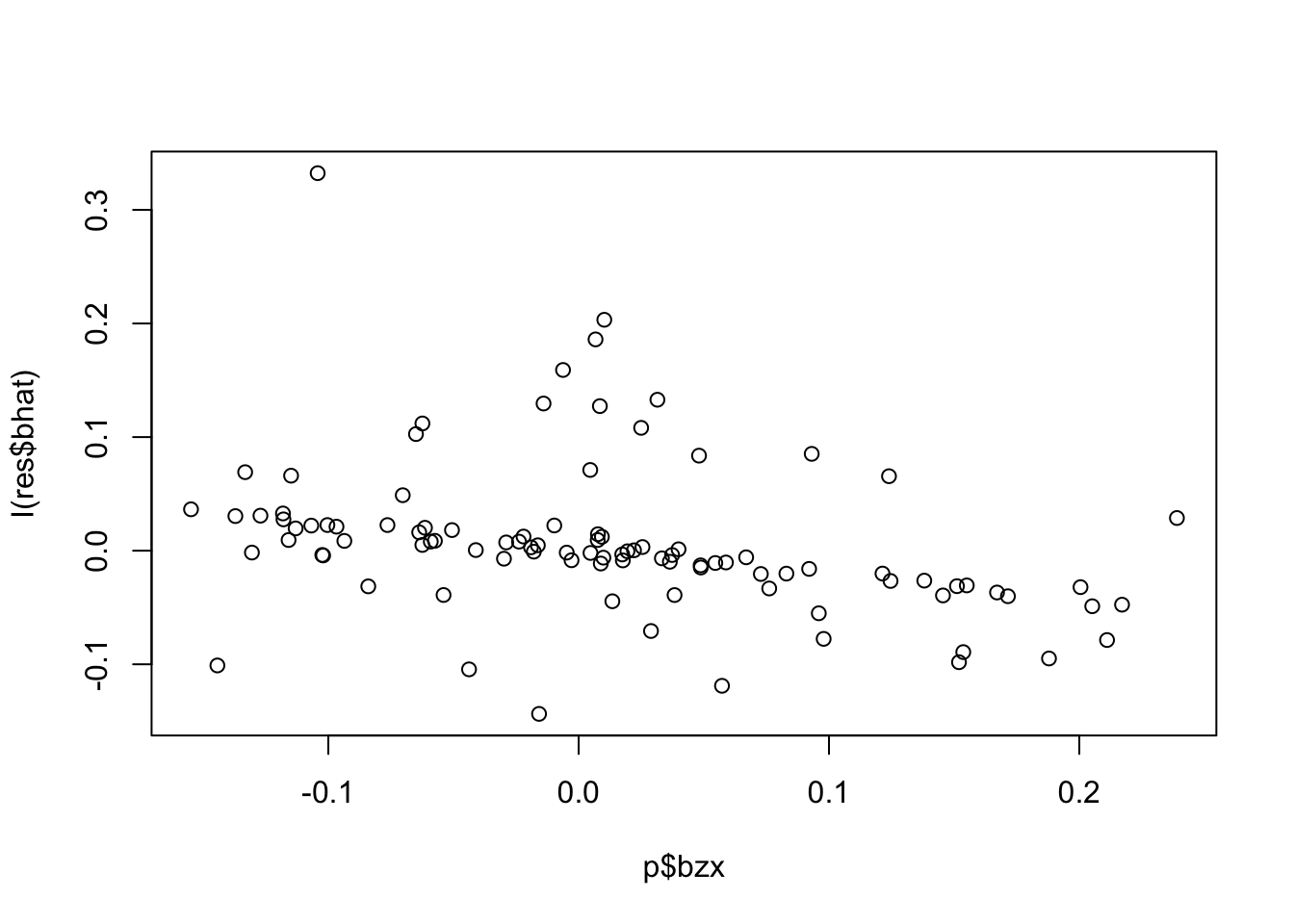
plot(I(res$bhat) ~ p$bzx)

summary(lm(I(res$bhat/p$bzx) ~ p$bzy))

Call:
lm(formula = I(res$bhat/p$bzx) ~ p$bzy)

Residuals:
     Min       1Q   Median       3Q      Max 
-27.8699  -0.5785  -0.4693  -0.1346  24.8711 

Coefficients:
            Estimate Std. Error t value Pr(>|t|)
(Intercept)   0.2642     0.5080   0.520    0.604
p$bzy        12.9040     7.8118   1.652    0.102

Residual standard error: 5.013 on 98 degrees of freedom
Multiple R-squared:  0.02709,   Adjusted R-squared:  0.01716 
F-statistic: 2.729 on 1 and 98 DF,  p-value: 0.1018
lapply(1:10, \(i) {
    p <- make_params(n=100000, nsnp=1, byu=)
})
[[1]]
[[1]]$nsnp
[1] 1

[[1]]$prop_pleio
[1] 0.5

[[1]]$n
[1] 1e+05

[[1]]$bxy
[1] 0.5

[[1]]$bxz
[1] 0.5

[[1]]$byu
[1] 0.5

[[1]]$bxu
[1] 0.5

[[1]]$bzx
[1] -0.003461206

[[1]]$bzy
[1] 0.07161975


[[2]]
[[2]]$nsnp
[1] 1

[[2]]$prop_pleio
[1] 0.5

[[2]]$n
[1] 1e+05

[[2]]$bxy
[1] 0.5

[[2]]$bxz
[1] 0.5

[[2]]$byu
[1] 0.5

[[2]]$bxu
[1] 0.5

[[2]]$bzx
[1] 0.002261778

[[2]]$bzy
[1] 0.08563668


[[3]]
[[3]]$nsnp
[1] 1

[[3]]$prop_pleio
[1] 0.5

[[3]]$n
[1] 1e+05

[[3]]$bxy
[1] 0.5

[[3]]$bxz
[1] 0.5

[[3]]$byu
[1] 0.5

[[3]]$bxu
[1] 0.5

[[3]]$bzx
[1] -0.08561653

[[3]]$bzy
[1] -0.1109887


[[4]]
[[4]]$nsnp
[1] 1

[[4]]$prop_pleio
[1] 0.5

[[4]]$n
[1] 1e+05

[[4]]$bxy
[1] 0.5

[[4]]$bxz
[1] 0.5

[[4]]$byu
[1] 0.5

[[4]]$bxu
[1] 0.5

[[4]]$bzx
[1] 0.01167803

[[4]]$bzy
[1] 0


[[5]]
[[5]]$nsnp
[1] 1

[[5]]$prop_pleio
[1] 0.5

[[5]]$n
[1] 1e+05

[[5]]$bxy
[1] 0.5

[[5]]$bxz
[1] 0.5

[[5]]$byu
[1] 0.5

[[5]]$bxu
[1] 0.5

[[5]]$bzx
[1] -0.01332658

[[5]]$bzy
[1] -0.1227844


[[6]]
[[6]]$nsnp
[1] 1

[[6]]$prop_pleio
[1] 0.5

[[6]]$n
[1] 1e+05

[[6]]$bxy
[1] 0.5

[[6]]$bxz
[1] 0.5

[[6]]$byu
[1] 0.5

[[6]]$bxu
[1] 0.5

[[6]]$bzx
[1] -0.1227617

[[6]]$bzy
[1] 0


[[7]]
[[7]]$nsnp
[1] 1

[[7]]$prop_pleio
[1] 0.5

[[7]]$n
[1] 1e+05

[[7]]$bxy
[1] 0.5

[[7]]$bxz
[1] 0.5

[[7]]$byu
[1] 0.5

[[7]]$bxu
[1] 0.5

[[7]]$bzx
[1] -0.0732307

[[7]]$bzy
[1] -0.01038855


[[8]]
[[8]]$nsnp
[1] 1

[[8]]$prop_pleio
[1] 0.5

[[8]]$n
[1] 1e+05

[[8]]$bxy
[1] 0.5

[[8]]$bxz
[1] 0.5

[[8]]$byu
[1] 0.5

[[8]]$bxu
[1] 0.5

[[8]]$bzx
[1] 0.0482732

[[8]]$bzy
[1] -0.02041057


[[9]]
[[9]]$nsnp
[1] 1

[[9]]$prop_pleio
[1] 0.5

[[9]]$n
[1] 1e+05

[[9]]$bxy
[1] 0.5

[[9]]$bxz
[1] 0.5

[[9]]$byu
[1] 0.5

[[9]]$bxu
[1] 0.5

[[9]]$bzx
[1] -0.05866098

[[9]]$bzy
[1] -0.07838496


[[10]]
[[10]]$nsnp
[1] 1

[[10]]$prop_pleio
[1] 0.5

[[10]]$n
[1] 1e+05

[[10]]$bxy
[1] 0.5

[[10]]$bxz
[1] 0.5

[[10]]$byu
[1] 0.5

[[10]]$bxu
[1] 0.5

[[10]]$bzx
[1] 0.009131354

[[10]]$bzy
[1] 0.1122955

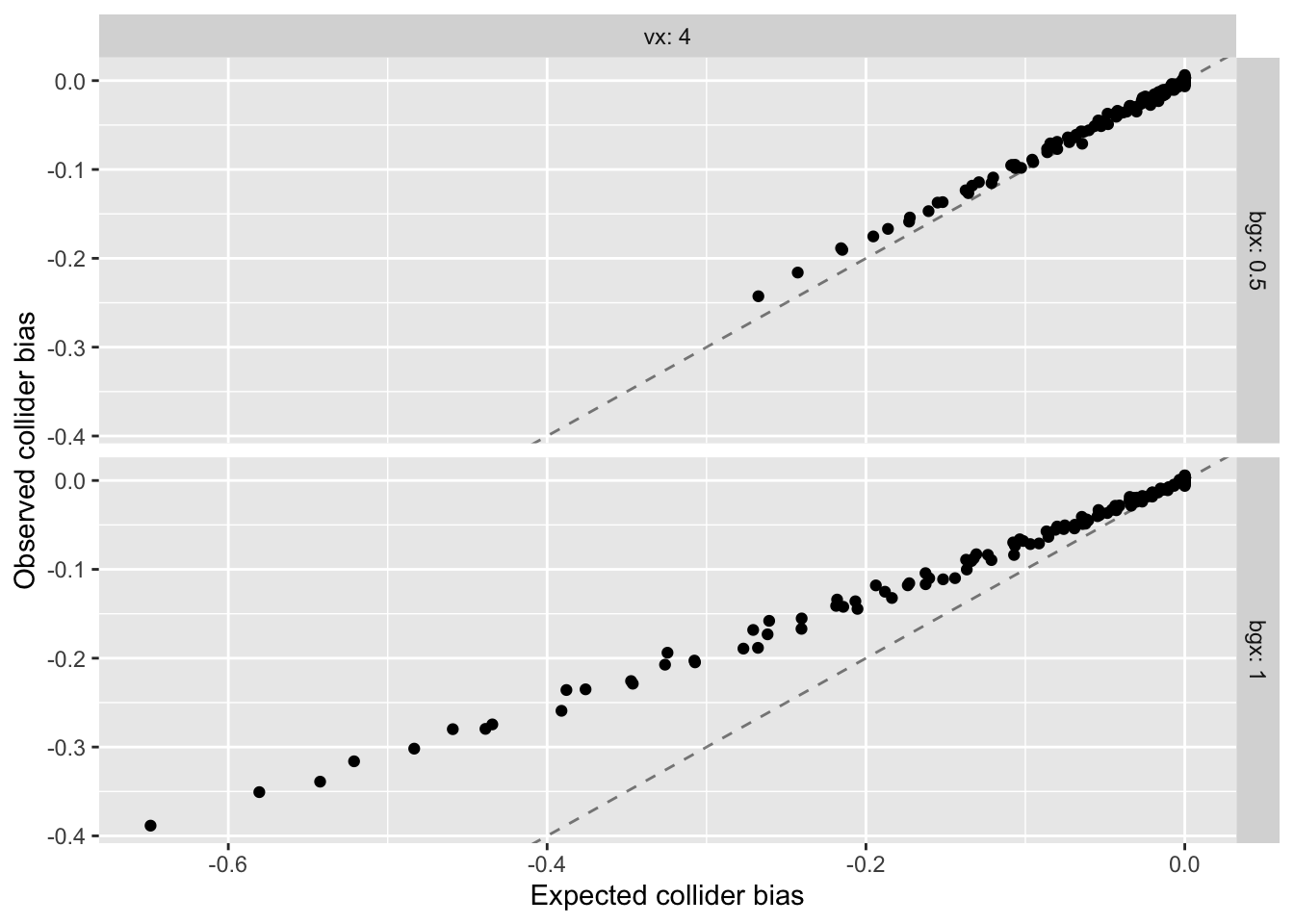
Expected collider bias = buy * bux / (bux^2 + var(x)) * bgx

sim <- function(buy=0.1, bux=0.1, vx=4, bgx=1) {
    n <- 100000
    u <- rnorm(n)
    g <- rnorm(n)
    gpred <- bgx * g
    uxpred <- bux * u
    resid <- rnorm(n, 0, sqrt(vx - var(gpred)) - var(uxpred))
    x <- gpred + uxpred + resid
    y <- buy * u + rnorm(n)
    cond <- residuals(lm(y ~ x))
    bhat <- lm(cond ~ g)$coef[2]
    exp <- -buy * bux / (bux^2 + var(resid)) * bgx
    tibble(
        buy=buy, bux=bux, vx=vx, bgx=bgx,
        varx=var(x), varu=var(u), varg=var(g),
        exp=exp, obs=bhat
    )
}

param <- expand.grid(
    buy=seq(0, 1, by=0.1),
    bux=seq(0, 1, by=0.1),
    vx=c(4),
    bgx=c(0.5, 1)
)

theoretical_res <- lapply(1:nrow(param), \(i) {
    sim(param$buy[i], param$bux[i], param$vx[i], param$bgx[i])
}) %>% bind_rows()

ggplot(theoretical_res, aes(x=exp, y=obs)) +
    geom_point() +
    geom_abline(slope=1, intercept=0, linetype="dashed", alpha=0.5) +
    facet_grid(bgx ~ vx, labeller = label_both) +
    labs(x="Expected collider bias", y="Observed collider bias")

In MR there is a question of how much horizontal pleiotropy is going to bias the IV estimate. I am starting to have the opinion that when you have a large number of SNPs, there are two classes of pleiotropy to be concerned about. 1) The SNP impacts Y through multiple independent paths, i.e. it is biologically complex; 2) The SNP more influences a confounder of X and Y, and arises as an instrument for Y.

One way to estimate the extent of (1) happening, would be to test if SNPs associate with Y conditional on X. A big problem with this approach is that X and Y are typically confounded, so conditioning on X will induce an association between the SNP and Y through the backdoor path via the confounder. But this bias would be a constant bias * the bgx effect, so it could be possible to (a) determine the extent of confounding and (b) determine the extent of deviation of all SNPs from the expected collider effect.
sessionInfo()
R version 4.6.0 (2026-04-24)
Platform: aarch64-apple-darwin23
Running under: macOS Sequoia 15.2

Matrix products: default
BLAS:   /Library/Frameworks/R.framework/Versions/4.6/Resources/lib/libRblas.0.dylib 
LAPACK: /Library/Frameworks/R.framework/Versions/4.6/Resources/lib/libRlapack.dylib;  LAPACK version 3.12.1

locale:
[1] en_US.UTF-8/en_US.UTF-8/en_US.UTF-8/C/en_US.UTF-8/en_US.UTF-8

time zone: Europe/London
tzcode source: internal

attached base packages:
[1] stats     graphics  grDevices utils     datasets  methods   base     

other attached packages:
 [1] here_1.0.2      furrr_0.4.0     future_1.70.0   lubridate_1.9.5
 [5] forcats_1.0.1   stringr_1.6.0   dplyr_1.2.1     purrr_1.2.2    
 [9] readr_2.2.0     tidyr_1.3.2     tibble_3.3.1    ggplot2_4.0.3  
[13] tidyverse_2.0.0

loaded via a namespace (and not attached):
 [1] gtable_0.3.6       jsonlite_2.0.0     compiler_4.6.0     tidyselect_1.2.1  
 [5] parallel_4.6.0     globals_0.19.1     scales_1.4.0       yaml_2.3.12       
 [9] fastmap_1.2.0      R6_2.6.1           labeling_0.4.3     generics_0.1.4    
[13] knitr_1.51         htmlwidgets_1.6.4  rprojroot_2.1.1    pillar_1.11.1     
[17] RColorBrewer_1.1-3 tzdb_0.5.0         rlang_1.2.0        stringi_1.8.7     
[21] xfun_0.57          S7_0.2.2           otel_0.2.0         timechange_0.4.0  
[25] cli_3.6.6          withr_3.0.2        magrittr_2.0.5     digest_0.6.39     
[29] grid_4.6.0         hms_1.1.4          lifecycle_1.0.5    vctrs_0.7.3       
[33] evaluate_1.0.5     glue_1.8.1         listenv_1.0.0      farver_2.1.2      
[37] codetools_0.2-20   parallelly_1.47.0  rmarkdown_2.31     tools_4.6.0       
[41] pkgconfig_2.0.3    htmltools_0.5.9