Shared modules across traits using gpmap

Use the GPMap pleiotropy profiles to find biological modules for a trait (univariate case) or shared/distinct for a pair of traits (bivariate case).

Univariate case

For a set of SNPs for a trait, I want to use GPMap pleiotropy profiles to cluster those SNPs due to their biological effects on the trait.

1. Construct the pleiotropy matrix

Suppose a target trait has \(n_{\text{snp}}\) associated variants.

For each SNP (j), extract its effects on all GPMap traits with at least one pleiotropic relationship to give

\[ X_{tj} \]

where:

• \(t = 1,\ldots,n_{\text{trait}}\) indexes GPMap traits
• \(j = 1,\ldots,n_{\text{snp}}\) indexes SNPs
• \(X_{tj}\) is the signed association statistic (e.g. Z-score) between SNP \(j\) and trait \(t\)

Each column of \(X\) represents the pleiotropic profile of a SNP.

---

2. Orient profiles relative to the target trait

Let

\[ z_j \]

be the signed effect of SNP \(j\) on the target trait.

To make all profiles relative to increasing liability for the target trait, define:

\[ X^*_{tj} = z_j X_{tj} \]

or alternatively

\[ X^*_{tj} = \operatorname{sign}(z_j) X_{tj} \]

The resulting matrix encodes whether a SNP’s effects on other traits are aligned or opposed to its effect on the target trait.

Interpretation:

• Positive values indicate agreement with the target trait direction.
• Negative values indicate opposition to the target trait direction.
• Larger magnitudes indicate stronger evidence.

---

3. Calculate SNP–SNP similarity

Each SNP is represented by a column vector:

\[ x^*_j \]

A similarity matrix can be constructed as:

\[ S = {X^*}^{\top}X^* \]

where

\[ S_{jk} = {x^*_j}^{\top}x^*_k \]

measures similarity between the target-oriented pleiotropic profiles of SNPs (j) and (k).

In practice, cosine similarity or correlation may be preferable:

\[ S_{jk} = \frac{{x^*_j}^{\top}x^*_k}{|x^*_j||x^*_k|} \]

to avoid dominance by highly pleiotropic variants.

---

4. Cluster SNPs

Apply a clustering algorithm to the similarity matrix e.g. 

• Hierarchical clustering
• Spectral clustering
• Community detection on a similarity graph
• Gaussian mixture models in latent space

The resulting clusters represent groups of SNPs with similar pleiotropic signatures.

---

5. Interpret biological modules

Some approaches

• For each cluster get a ‘score’ for how strongly each trait associates with the cluster - this will allow us to rank the relevance of traits to each cluster
• Get a list of genes based on eqtls for the SNPs in the cluster and do pathway / gene set enrichment
• Do some sort of topic modelling of all the traits that associate with a cluster

Simulation for univariate case

set.seed(1)

# Dimensions
n_trait <- 80   # GPMap traits
n_snp   <- 60   # SNPs for target trait
K       <- 3    # biological modules

# Trait-module loadings
B <- matrix(0, n_trait, K)
B[1:25, 1]  <- 1   # module 1 traits
B[26:50, 2] <- 1   # module 2 traits
B[51:80, 3] <- 1   # module 3 traits

# SNP-module membership
M <- matrix(0, n_snp, K)
M[1:20, 1]  <- 1
M[21:40, 2] <- 1
M[41:60, 3] <- 1

# Signed target-trait effects
z_target <- rnorm(n_snp, mean = 5, sd = 1)

# Make one module protective/opposite direction
z_target[21:40] <- -z_target[21:40]

# Pleiotropy matrix: rows = GPMap traits, columns = SNPs
X <- B %*% t(M) + matrix(rnorm(n_trait * n_snp, 0, 0.5), n_trait, n_snp)

# Orient pleiotropy relative to the target trait
X_star <- sweep(X, 2, sign(z_target), `*`)

# Cosine similarity between SNP pleiotropy profiles
cosine_sim <- function(A) {
  A_norm <- sweep(A, 2, sqrt(colSums(A^2)), `/`)
  t(A_norm) %*% A_norm
}

S <- cosine_sim(X_star)

# Cluster SNPs
hc <- hclust(as.dist(1 - S), method = "average")

# Visualise similarity matrix
heatmap(
  S,
  Rowv = as.dendrogram(hc),
  Colv = as.dendrogram(hc),
  scale = "none",
  main = "SNP similarity based on target-oriented pleiotropy",
  xlab = "SNPs",
  ylab = "SNPs"
)

# Recover clusters
clusters <- cutree(hc, k = K)

# Compare inferred clusters to true modules
true_module <- rep(c("module_1", "module_2", "module_3"), each = 20)

table(
  true_module = true_module,
  inferred_cluster = clusters
)

           inferred_cluster
true_module  1  2  3
   module_1 20  0  0
   module_2  0 20  0
   module_3  0  0 20

# Average target-oriented pleiotropy profile per inferred cluster
cluster_profiles <- sapply(sort(unique(clusters)), function(cl) {
  rowMeans(X_star[, clusters == cl, drop = FALSE])
})

# Traits most strongly associated with each inferred module
apply(cluster_profiles, 2, function(x) {
  head(order(abs(x), decreasing = TRUE), 10)
})

      [,1] [,2] [,3]
 [1,]   10   32   78
 [2,]    5   34   53
 [3,]    2   33   72
 [4,]    6   41   71
 [5,]   25   28   54
 [6,]   17   31   56
 [7,]    3   29   67
 [8,]   20   47   69
 [9,]   11   27   66
[10,]    8   43   68

Bivariate case

For two target traits, SNPs can be represented by their pleiotropic effects across all traits in the genotype–phenotype map (GPMap). Variants that exhibit similar pleiotropic profiles are hypothesised to influence disease risk through similar biological mechanisms.

The objective is to identify:

• Biological modules shared between the two traits.
• Biological modules unique to each trait.
• Biological modules that have opposite consequences for the two traits.

---

1. Construct pleiotropy matrices

Suppose trait 1 has \(n_1\) associated variants and trait 2 has \(n_2\) associated variants.

For each SNP, extract its effects on all GPMap traits that associate with at least one of the two traits. This gives two pleiotropy matrices:

Define:

\[ X_1 \in \mathbb{R}^{n_{\text{trait}} \times n_1} \]

and

\[ X_2 \in \mathbb{R}^{n_{\text{trait}} \times n_2} \]

where

\[ X_{1,tj} \]

and

\[ X_{2,tk} \]

represent the signed association statistic (e.g. Z-score) between a SNP and GPMap trait \(t\).

Each column corresponds to the pleiotropic profile of a SNP.

---

2. Orient profiles relative to each target trait

Let

\[ z_{1j} \]

denote the effect of SNP \(j\) on trait 1 and

\[ z_{2k} \]

denote the effect of SNP \(k\) on trait 2.

Orient all pleiotropic effects relative to increasing liability for the corresponding target trait:

\[ X^*_{1,tj} = \operatorname{sign}(z_{1j}) X_{1,tj} \]

\[ X^*_{2,tk} = \operatorname{sign}(z_{2k}) X_{2,tk} \]

The resulting matrices encode whether a SNP’s effects on other traits are aligned or opposed to increased risk of the target trait.

---

3. Calculate cross-trait SNP similarity

For each SNP from trait 1 and each SNP from trait 2, compute similarity between their target-oriented pleiotropic profiles.

For example, using cosine similarity:

\[ S_{jk} = \frac{ {x^*_{1,j}}^\top x^*_{2,k} } { \|x^*_{1,j}\| \, \|x^*_{2,k}\| } \]

This yields

\[ S \in \mathbb{R}^{n_1 \times n_2} \]

where:

• Rows correspond to SNPs associated with trait 1.
• Columns correspond to SNPs associated with trait 2.

Large positive values indicate similar pleiotropic signatures.

Large negative values indicate similar biological programmes acting in opposite directions.

Values near zero indicate little evidence of shared function.

---

4. Identify shared biological modules

Cluster the similarity matrix \(S\) using:

• Hierarchical clustering
• Spectral clustering
• Community detection
• Matrix factorisation

Shared modules appear as blocks of elevated similarity between subsets of SNPs from both traits.

These blocks represent groups of variants that perturb similar downstream phenotypic systems.

5. Interpret biological modules

Some approaches

• For each cluster get a ‘score’ for how strongly each trait associates with the cluster - this will allow us to rank the relevance of traits to each cluster
• Get a list of genes based on eqtls for the SNPs in the cluster and do pathway / gene set enrichment
• Do some sort of topic modelling of all the traits that associate with a cluster

Example simulation

set.seed(1)

# Dimensions
n_trait <- 80     # GPMap pleiotropic traits
n1 <- 40          # SNPs for target trait 1
n2 <- 40          # SNPs for target trait 2
K <- 4            # latent biological modules

# Trait-module loadings: each module affects a subset of pleiotropic traits
B <- matrix(0, n_trait, K)
B[1:20, 1]  <- 1      # shared module A
B[21:40, 2] <- 1      # shared module B
B[41:60, 3] <- 1      # trait-1-specific module
B[61:80, 4] <- 1      # trait-2-specific module

# SNP-module memberships
M1 <- matrix(0, n1, K)
M2 <- matrix(0, n2, K)

M1[1:10, 1]  <- 1     # trait 1 SNPs in shared module A
M1[11:20, 2] <- 1     # trait 1 SNPs in shared module B
M1[21:40, 3] <- 1     # trait 1-specific SNPs

M2[1:10, 1]  <- 1     # trait 2 SNPs in shared module A
M2[11:20, 2] <- 1     # trait 2 SNPs in shared module B
M2[21:40, 4] <- 1     # trait 2-specific SNPs

# Allow some SNPs to have opposite target-trait direction
z1 <- rnorm(n1, mean = 5, sd = 1)
z2 <- rnorm(n2, mean = 5, sd = 1)

z1[11:20] <- -z1[11:20]   # module B has opposite direction for trait 1
z2[11:20] <-  z2[11:20]   # module B positive for trait 2

# Generate raw pleiotropy matrices
# rows = pleiotropic traits, columns = SNPs
X1 <- B %*% t(M1) + matrix(rnorm(n_trait * n1, 0, 0.5), n_trait, n1)
X2 <- B %*% t(M2) + matrix(rnorm(n_trait * n2, 0, 0.5), n_trait, n2)

# Target-oriented profiles
X1_star <- sweep(X1, 2, z1, `*`)
X2_star <- sweep(X2, 2, z2, `*`)

# Cross-trait similarity: SNPs from trait 1 vs SNPs from trait 2
cosine_sim <- function(A, B) {
  A_norm <- sweep(A, 2, sqrt(colSums(A^2)), `/`)
  B_norm <- sweep(B, 2, sqrt(colSums(B^2)), `/`)
  t(A_norm) %*% B_norm
}

S_raw  <- cosine_sim(X1, X2)
S_star <- cosine_sim(X1_star, X2_star)

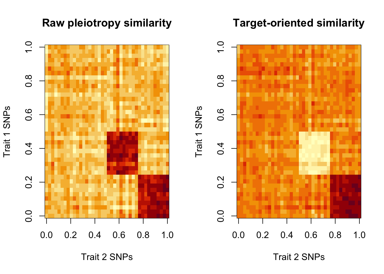
# Visualise
par(mfrow = c(1, 2))

image(
  S_raw[nrow(S_raw):1, ],
  main = "Raw pleiotropy similarity",
  xlab = "Trait 2 SNPs",
  ylab = "Trait 1 SNPs"
)

image(
  S_star[nrow(S_star):1, ],
  main = "Target-oriented similarity",
  xlab = "Trait 2 SNPs",
  ylab = "Trait 1 SNPs"
)

par(mfrow = c(1, 1))

# Cluster the target-oriented similarity matrix
hc1 <- hclust(dist(S_star))
hc2 <- hclust(dist(t(S_star)))

heatmap(
  S_star,
  Rowv = as.dendrogram(hc1),
  Colv = as.dendrogram(hc2),
  scale = "none",
  main = "Clustered SNP similarity: target-oriented profiles",
  xlab = "Trait 2 SNPs",
  ylab = "Trait 1 SNPs"
)

# Inspect average similarity by known module
module1 <- rep(c("shared_A", "shared_B", "trait1_specific"), c(10, 10, 20))
module2 <- rep(c("shared_A", "shared_B", "trait2_specific"), c(10, 10, 20))

aggregate_similarity <- outer(
  unique(module1),
  unique(module2),
  Vectorize(function(a, b) {
    mean(S_star[module1 == a, module2 == b])
  })
)

rownames(aggregate_similarity) <- unique(module1)
colnames(aggregate_similarity) <- unique(module2)

round(aggregate_similarity, 2)

                shared_A shared_B trait2_specific
shared_A            0.50    -0.01           -0.02
shared_B            0.01    -0.48           -0.01
trait1_specific     0.01    -0.02            0.02

---

sessionInfo()

R version 4.6.0 (2026-04-24)
Platform: aarch64-apple-darwin23
Running under: macOS Sequoia 15.2

Matrix products: default
BLAS:   /Library/Frameworks/R.framework/Versions/4.6/Resources/lib/libRblas.0.dylib 
LAPACK: /Library/Frameworks/R.framework/Versions/4.6/Resources/lib/libRlapack.dylib;  LAPACK version 3.12.1

locale:
[1] en_US.UTF-8/en_US.UTF-8/en_US.UTF-8/C/en_US.UTF-8/en_US.UTF-8

time zone: Europe/London
tzcode source: internal

attached base packages:
[1] stats     graphics  grDevices utils     datasets  methods   base     

loaded via a namespace (and not attached):
 [1] htmlwidgets_1.6.4 compiler_4.6.0    fastmap_1.2.0     cli_3.6.6        
 [5] tools_4.6.0       htmltools_0.5.9   otel_0.2.0        yaml_2.3.12      
 [9] rmarkdown_2.31    knitr_1.51        jsonlite_2.0.0    xfun_0.57        
[13] digest_0.6.39     rlang_1.2.0       evaluate_1.0.5