library(tidyverse)simulate_time_to_event <-function(liability, baseline_rate =0.1, shape =1) {#' Simulate time-to-event data based on individual liability#' #' @param liability Vector of individual liability values#' @param baseline_rate Baseline hazard rate (lambda parameter)#' @param shape Shape parameter for Weibull distribution (shape=1 gives exponential)#' @return Vector of simulated time to event for each individual n <-length(liability)# Convert liability to hazard rate (exponential relationship)# Higher liability = higher hazard = shorter time to event hazard_rate <- baseline_rate *exp(liability)# Scale parameter for Weibull (lambda = 1/scale) scale <-1/ hazard_rate# Simulate time to event using Weibull distribution# When shape=1, this is exponential distribution time_to_event <-rweibull(n, shape = shape, scale = scale)return(time_to_event)}# Example simulationset.seed(42)n_individuals <-1000# Simulate liability (e.g., genetic risk, standardized)liability <-rnorm(n_individuals, mean =0, sd =1)# Simulate time to eventtime_to_event <-simulate_time_to_event(liability, baseline_rate =0.1, shape =10)# Create dataframedf <-tibble(individual_id =1:n_individuals,liability = liability,time_to_event = time_to_event)
── Attaching core tidyverse packages ──────────────────────── tidyverse 2.0.0 ──
✔dplyr 1.1.4 ✔readr 2.2.0
✔forcats 1.0.1 ✔stringr 1.6.0
✔ggplot2 4.0.1 ✔tibble 3.3.0
✔lubridate 1.9.4 ✔tidyr 1.3.1
✔purrr 1.2.0
── Conflicts ────────────────────────────────────────── tidyverse_conflicts() ──
✖dplyr::filter() masks stats::filter()
✖dplyr::lag() masks stats::lag()
ℹ Use the conflicted package (<http://conflicted.r-lib.org/>) to force all conflicts to become errors
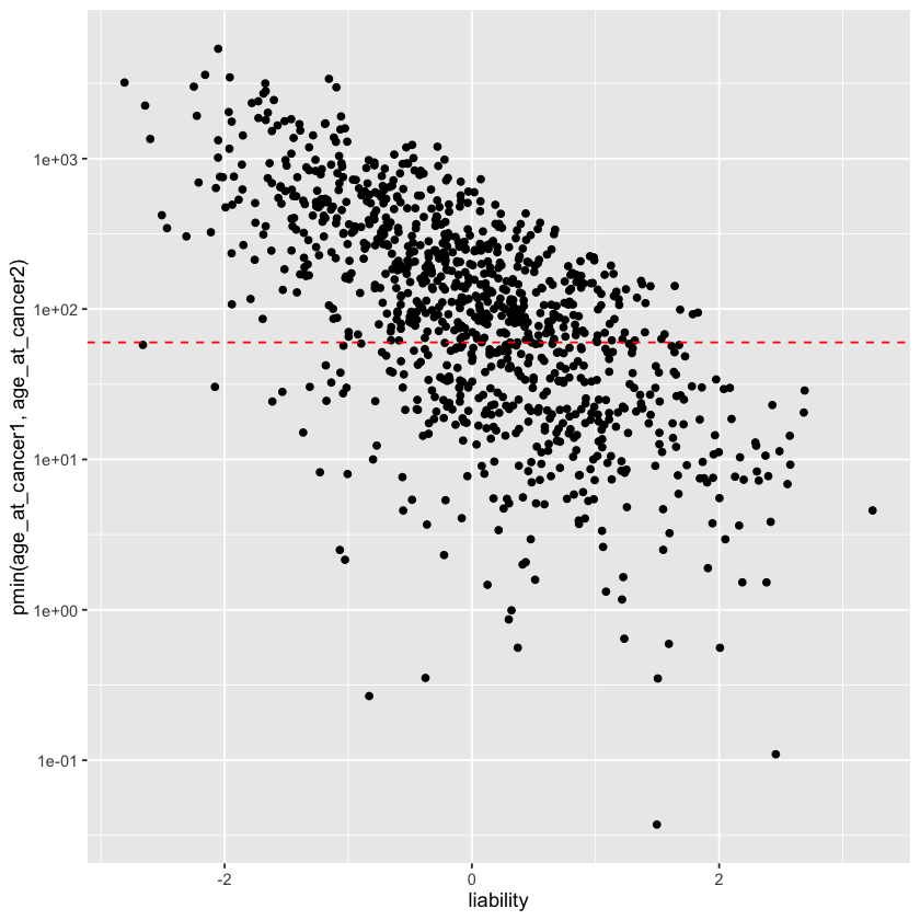
set.seed(123)n <-1000# Simulate genetic/environmental liability (standardized)liability <-rnorm(n, mean =0, sd =1)# For cancer with median onset around age 65-70:# baseline_rate = 0.015 gives expected time ~ 67 years for liability=0cancer_data <-tibble(person_id =1:n,liability = liability,age_at_cancer1 =simulate_time_to_event(liability, baseline_rate =0.003, shape =1),age_at_cancer2 =simulate_time_to_event(liability, baseline_rate =0.003, shape =1),diff =abs(age_at_cancer1 - age_at_cancer2),below_60 = age_at_cancer1 <60| age_at_cancer2 <60)str(cancer_data)
`summarise()` has grouped output by 'below_60'. You can override using the

`.groups` argument.
A grouped_df: 4 × 4
below_60
diff <= 5
n
prop
<lgl>
<lgl>
<int>
<dbl>
FALSE
FALSE
613
0.613
FALSE
TRUE
11
0.011
TRUE
FALSE
365
0.365
TRUE
TRUE
11
0.011
set.seed(123)n <-1000# Simulate genetic/environmental liability (standardized)liability <-rnorm(n, mean =0, sd =3)# For cancer with median onset around age 65-70:# baseline_rate = 0.015 gives expected time ~ 67 years for liability=0cancer_data <-tibble(person_id =1:n,liability = liability,age_at_cancer1 =simulate_time_to_event(liability, baseline_rate =0.003, shape =1),age_at_cancer2 =simulate_time_to_event(liability, baseline_rate =0.003, shape =1),diff =abs(age_at_cancer1 - age_at_cancer2),below_60 = age_at_cancer1 <60| age_at_cancer2 <60)cancer_data %>%group_by(below_60, diff <=5) %>%summarise(n =n(), prop=n()/nrow(cancer_data))
`summarise()` has grouped output by 'below_60'. You can override using the

`.groups` argument.
A grouped_df: 4 × 4
below_60
diff <= 5
n
prop
<lgl>
<lgl>
<int>
<dbl>
FALSE
FALSE
536
0.536
FALSE
TRUE
5
0.005
TRUE
FALSE
328
0.328
TRUE
TRUE
131
0.131
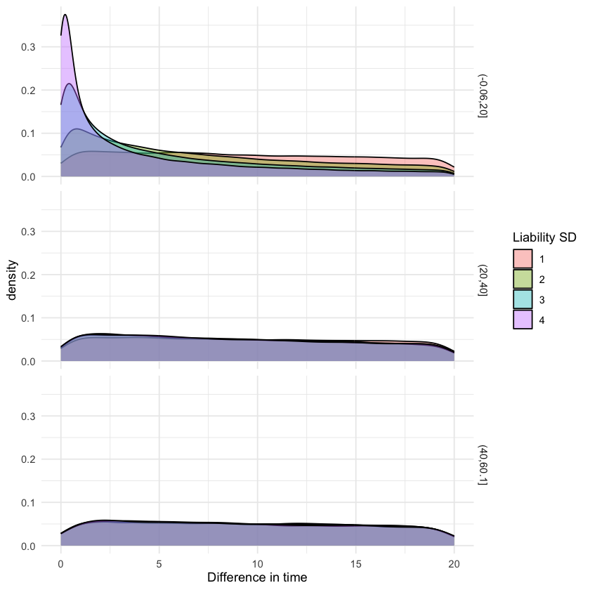
When the liability has a low variance (i.e. not contributing much to overall risk, most risk comes from chance), then bilateral cancer incidence within 5 years is at 1%.
When liability has a high variance (i.e. smaller chance component) then bilateral cancer incidence within 5 years is at 13%.
One way to determine if bilateral cancer is occurring more than expected is to look at familial rates. Suppose siblings share ~50% genetics and X% environmental liability, we can get expected and observed rates for bilateral cancer and sibling cancer.