Smoothing noisy age-stratified genetic effect estimates

We want to represent the pattern of how a SNP effect changes by age, however:

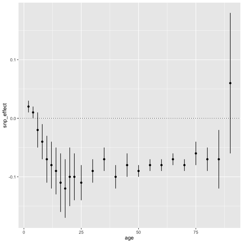
Effect estimates can be erratic when standard errors are large
Using z-scores can be more influenced by different sample sizes across ages

Ideally we would use smoothed betas to solve both of these issues.

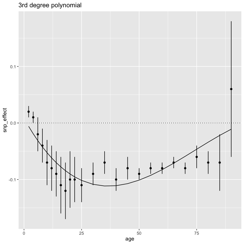
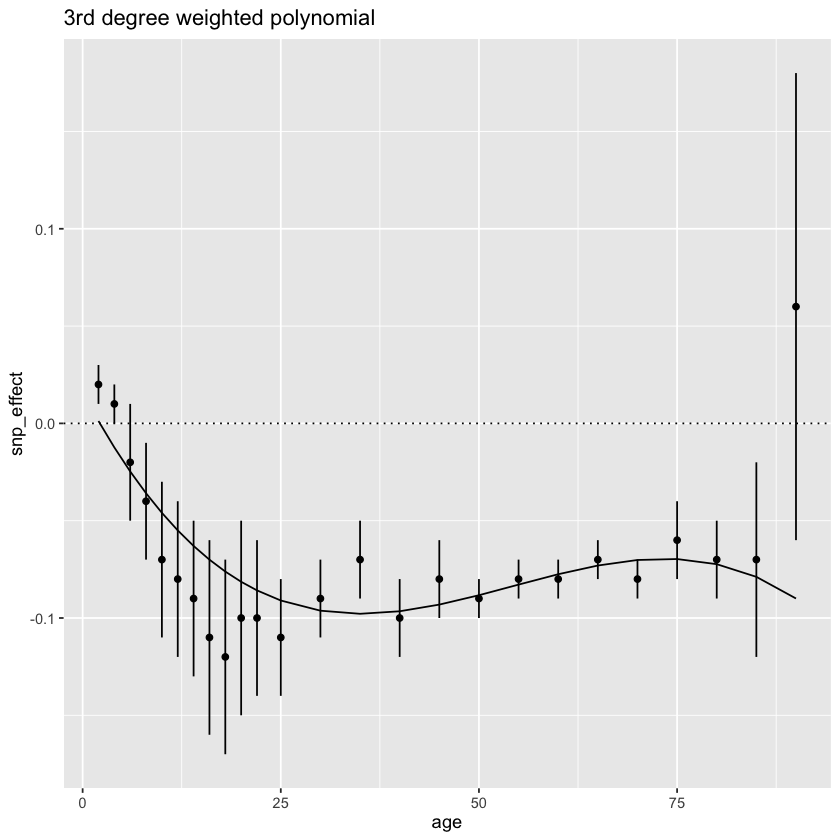
Polynomial meta regression can handle sample overlap which is ideal for hypothesis testing, but imposes a functional form which won’t represent the age-trajectory patterns accurately
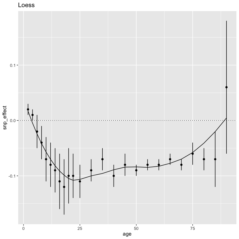
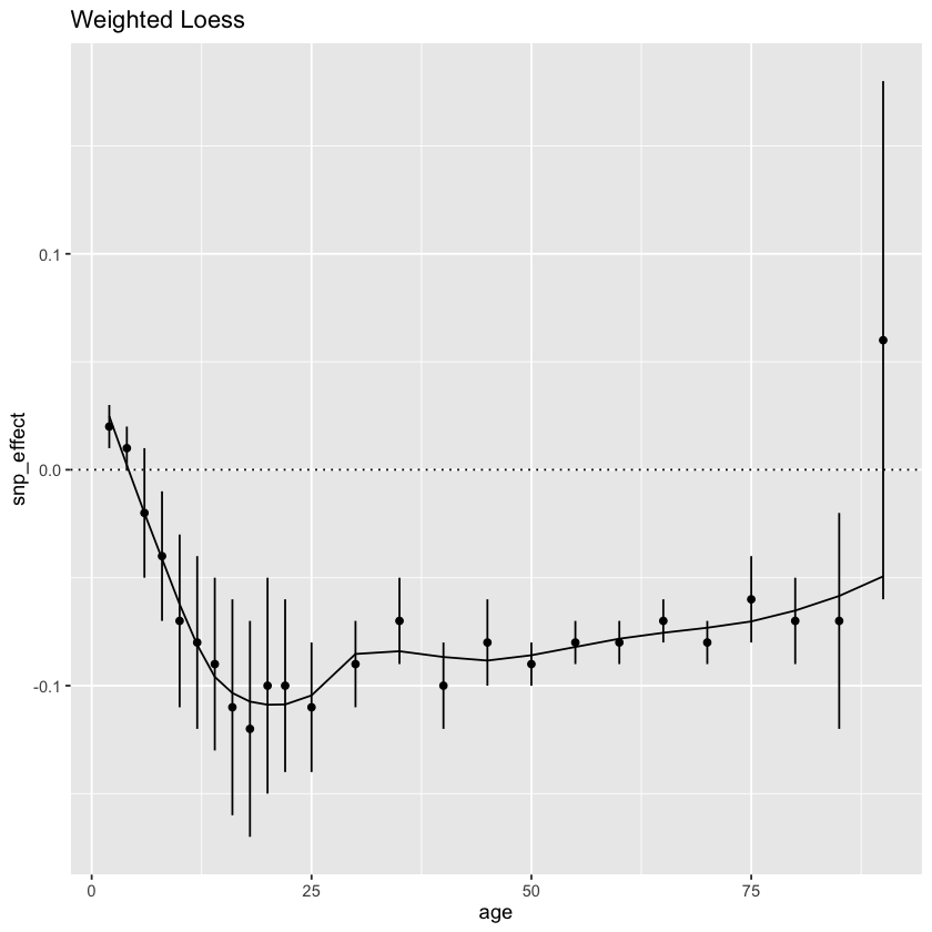
Non-parametric smoothing (e.g. LOESS smoothers) can do a better job of capturing the shape without having a statistically clear interpretation

This basic analysis explores how to get smoothed betas.

Approximate the age-stratified effect estimate results for the FTO variant on BMI
However I did artificially make the very imprecise estimate for age 90 to be slightly off the obvious trend to try to capture

library(here)
dat <- read.csv(here("posts", "2026-03-17-gxage-smoother", "data.csv"))
str(dat)

'data.frame':   25 obs. of  5 variables:
 $ age       : int  2 4 6 8 10 12 14 16 18 20 ...
 $ snp_effect: num  0.02 0.01 -0.02 -0.04 -0.07 -0.08 -0.09 -0.11 -0.12 -0.1 ...
 $ lower_ci  : num  0.01 0 -0.05 -0.07 -0.11 -0.12 -0.13 -0.16 -0.17 -0.15 ...
 $ upper_ci  : num  0.03 0.02 0.01 -0.01 -0.03 -0.04 -0.05 -0.06 -0.07 -0.05 ...
 $ se        : num  0.0153 0.0153 0.0153 0.0153 0.0204 0.0204 0.0204 0.0255 0.0255 0.0255 ...

library(ggplot2)
library(dplyr)
dat %>% ggplot(., aes(x=age, y=snp_effect)) +
geom_point() +
geom_errorbar(width=0, aes(ymin = lower_ci, ymax = upper_ci)) +
geom_hline(yintercept=0, linetype="dotted")

Use LOESS to get the smoothed line through these points, with or without weights

l1 <- loess(snp_effect ~ age, data=dat)
dat$loess <- predict(l1, span=0.4)
l2 <- loess(snp_effect ~ age, data=dat, weight=1/dat$se^2, span=0.4)
dat$loessw <- predict(l2)
l3 <- lm(snp_effect ~ poly(age, 3), dat)
dat$poly3 <- predict(l3)
l4 <- lm(snp_effect ~ poly(age, 3), dat, weight=1/dat$se^2)
dat$poly3w <- predict(l4)

dat %>% ggplot(., aes(x=age, y=snp_effect)) +
geom_point() +
geom_errorbar(width=0, aes(ymin = lower_ci, ymax = upper_ci)) +
geom_line(aes(y=poly3)) +
labs(title="3rd degree polynomial") +
geom_hline(yintercept=0, linetype="dotted")

dat %>% ggplot(., aes(x=age, y=snp_effect)) +
geom_point() +
geom_errorbar(width=0, aes(ymin = lower_ci, ymax = upper_ci)) +
geom_line(aes(y=poly3w)) +
labs(title="3rd degree weighted polynomial") +
geom_hline(yintercept=0, linetype="dotted")

dat %>% ggplot(., aes(x=age, y=snp_effect)) +
geom_point() +
geom_errorbar(width=0, aes(ymin = lower_ci, ymax = upper_ci)) +
geom_line(aes(y=loess)) +
labs(title="Loess") +
geom_hline(yintercept=0, linetype="dotted")

dat %>% ggplot(., aes(x=age, y=snp_effect)) +
geom_point() +
geom_errorbar(width=0, aes(ymin = lower_ci, ymax = upper_ci)) +
geom_line(aes(y=loessw)) +
labs(title="Weighted Loess") +
geom_hline(yintercept=0, linetype="dotted")