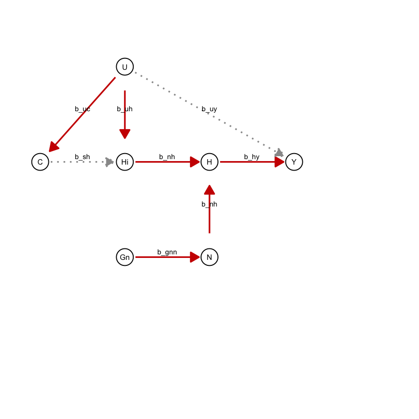
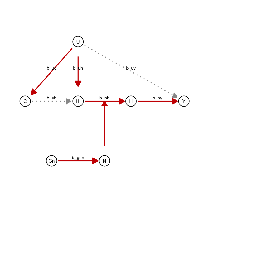
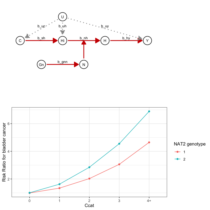
draw_dag <- function(b_hy, b_uy, b_sh, b_nh, b_gcc, b_gis, b_gnn, b_us, b_uc, b_uh) {
nodes <- tibble::tribble(
~node, ~x, ~y,
# "Gc", 1, 4,
# "Gi", 1, 3,
"Gn", 3, 2,
"U", 3, 4,
"C", 1, 3,
"N", 5, 2,
"Hi", 3, 3,
"H", 5, 3,
"Y", 7, 3
)
edges <- tibble::tribble(
~from, ~to, ~beta, ~label, ~curv,
# "Gc", "C", b_gcc, "b_gcc", 0.00,
# "Gi", "C", b_gis, "b_gis", 0,
# "U", "C", b_us, "b_us", 0.20,
"U", "C", b_uc, "b_uc", 0,
"Gn", "N", b_gnn, "b_gnn", 0.00,
"C", "Hi", b_sh, "b_sh", 0.00,
"U", "Hi", b_uh, "b_uh", 0.00,
"Hi", "H", b_nh, "b_nh", 0.00,
"N", "H", b_nh, "b_nh", 0,
"H", "Y", b_hy, "b_hy", 0.00,
"U", "Y", b_uy, "b_uy", 0
) %>%
dplyr::mutate(
sign_type = dplyr::case_when(
beta > 0 ~ "pos",
beta < 0 ~ "neg",
TRUE ~ "null"
),
col = dplyr::case_when(
sign_type == "pos" ~ "red3",
sign_type == "neg" ~ "blue3",
TRUE ~ "grey60"
),
lty = ifelse(sign_type == "null", "dotted", "solid")
) %>%
dplyr::left_join(nodes, by = c("from" = "node")) %>%
dplyr::left_join(nodes, by = c("to" = "node"), suffix = c("", "end")) %>%
dplyr::mutate(
# Shorten arrows to stop at node edges
dx = xend - x,
dy = yend - y,
length = sqrt(dx^2 + dy^2),
# Shorten by 0.25 units at each end (approximate node radius)
x = x + 0.25 * dx / length,
y = y + 0.25 * dy / length,
xend = xend - 0.25 * dx / length,
yend = yend - 0.25 * dy / length
)
# Split edges into straight and curved
edges_straight <- edges %>% dplyr::filter(curv == 0)
edges_curved <- edges %>% dplyr::filter(curv != 0)
p <- ggplot2::ggplot()
# Add straight edges
if (nrow(edges_straight) > 0) {
p <- p + ggplot2::geom_segment(
data = edges_straight,
ggplot2::aes(
x = x, y = y, xend = xend, yend = yend,
color = col, linetype = lty
),
arrow = grid::arrow(length = grid::unit(0.4, "cm"), type = "closed"),
linewidth = 0.9
)
}
# Add curved edges (one layer per unique curvature value)
if (nrow(edges_curved) > 0) {
for (curv_val in unique(edges_curved$curv)) {
edges_subset <- edges_curved %>% dplyr::filter(curv == curv_val)
p <- p + ggplot2::geom_curve(
data = edges_subset,
ggplot2::aes(
x = x, y = y, xend = xend, yend = yend,
color = col, linetype = lty
),
curvature = curv_val,
arrow = grid::arrow(length = grid::unit(0.4, "cm"), type = "closed"),
linewidth = 0.9
)
}
}
p <- p +
ggplot2::geom_text(
data = edges,
ggplot2::aes(
x = (x + xend) / 2,
y = (y + yend) / 2,
label = label
),
size = 3, vjust = -0.6
) +
ggplot2::geom_point(
data = nodes,
ggplot2::aes(x = x, y = y),
size = 9, shape = 21, fill = "white", color = "black", stroke = 0.8
) +
ggplot2::geom_text(
data = nodes,
ggplot2::aes(x = x, y = y, label = node),
size = 3.2
) +
ggplot2::scale_color_identity() +
ggplot2::scale_linetype_identity() +
ggplot2::theme_void() +
ggplot2::coord_cartesian(xlim = c(0.5, 9.5), ylim = c(0.5, 4.5))
return(p)
}
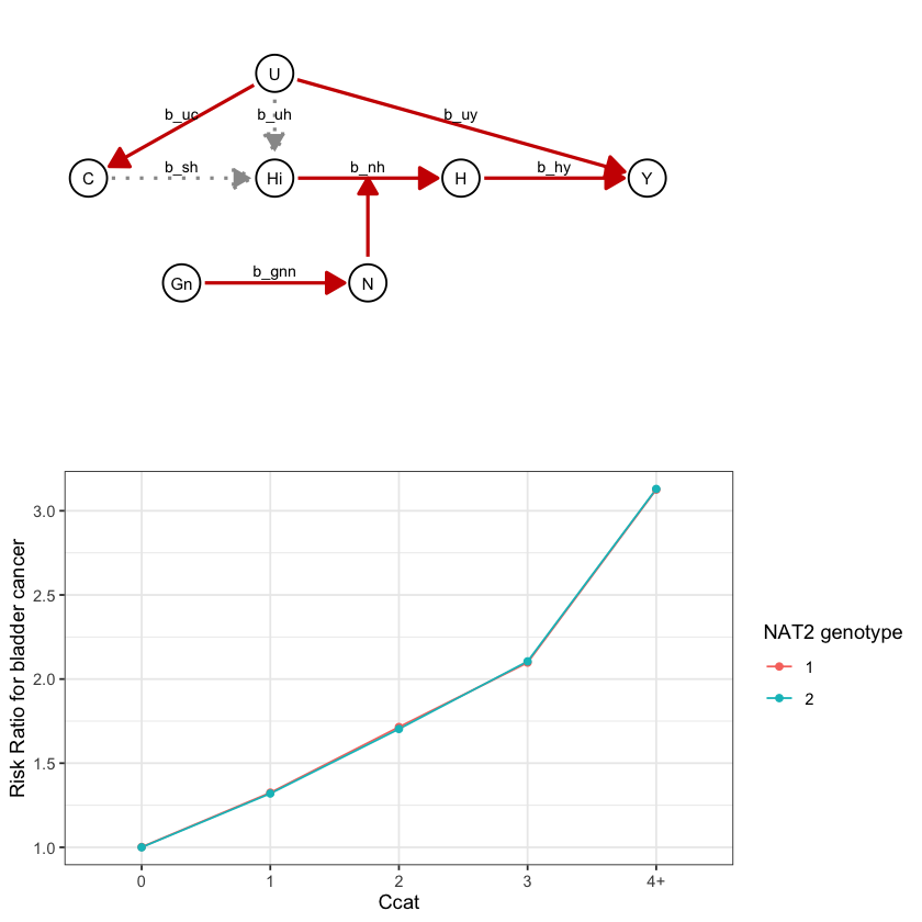
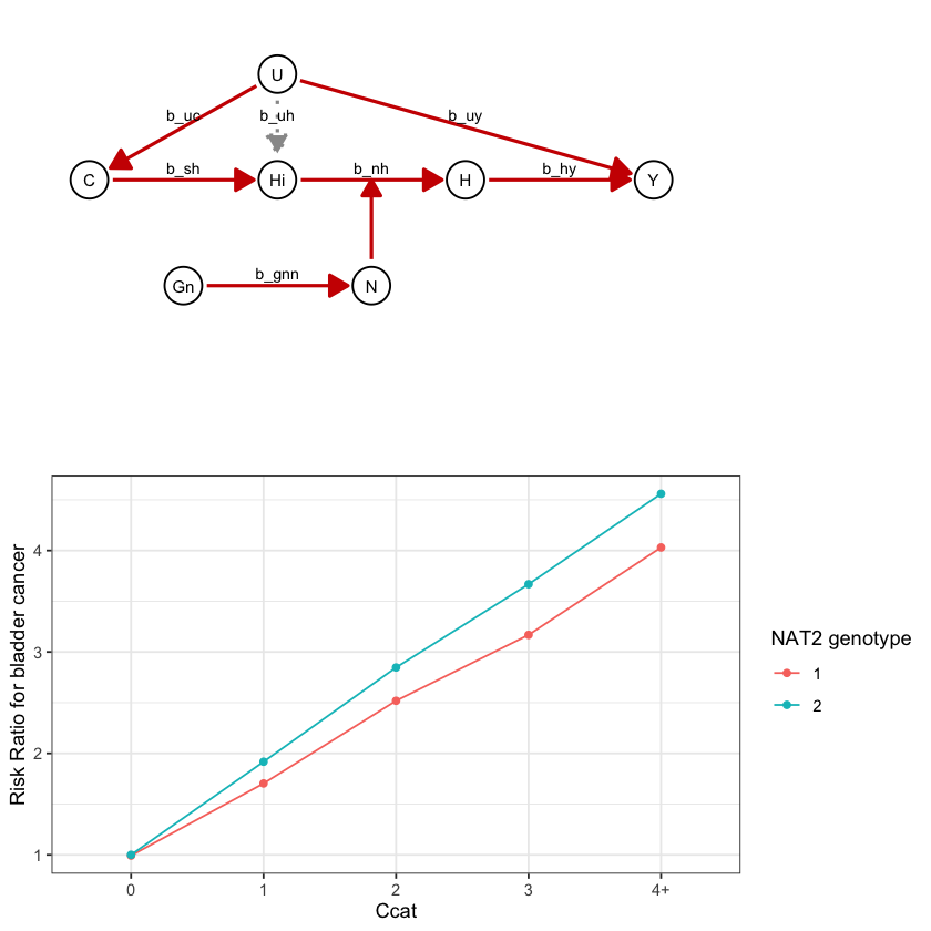
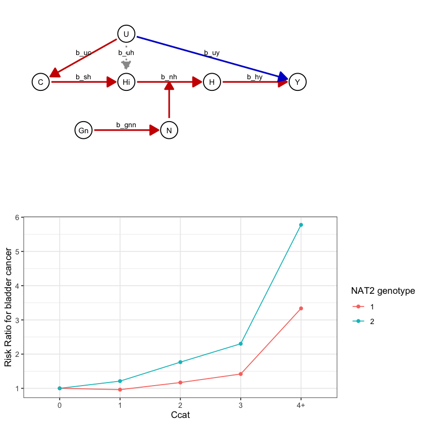
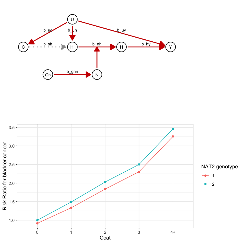
a <- draw_dag(
b_hy = 2,
b_uy = 0,
b_sh = 0,
b_nh = 0.2,
b_gcc = 1.0,
b_gis = 1.0,
b_gnn = 0.4,
b_us = 2,
b_uc = 2,
b_uh = 3
)
class(a)
a