The following objects are masked from 'package:stats':

    filter, lag
The following objects are masked from 'package:base':

    intersect, setdiff, setequal, union
library(simsurv)library(survival)library(boot)
Attaching package: 'boot'
The following object is masked from 'package:survival':

    aml
set.seed(123)
Manually estimating power
Suppose I want to know the power of a linear regression model through simulation. Generate simulated data to match what I see in my real analysis - the data generating model (DGM)
Here we have a variable x and y, both have variance of 1
There is some sample size n
But I don’t know the effect size of x on y
I will be varying the effect size (beta) to see how it affects power
dgm <-function(n =30, beta =0.2) { x <-rnorm(n)# We want the variance of y to be 1, so we just add enough noise on top of x*beta y <- beta * x +rnorm(n, sd =sqrt(1- beta^2))tibble(x = x, y = y)}
Now that I’ve generated the data to mimic my real analysis, I need to estimate the effect of x on y in the same way that I would in the real analysis
estimation <-function(data) { model <-lm(y ~ x, data = data)summary(model)$coefficients[2, 4] # p-value for the slope}
Finally, I need to run this across lots of different potential values of beta and n, to see the average power.
Power depends on the significance threshold (alpha). If I simulate a null where beta = 0, then I want power to equal the significance threshold
power_simulation <-function(nsim =1000, n =c(30, 50, 70), beta =c(0, 0.2, 0.4), alpha =0.05) { params <-expand.grid(n = n, beta = beta, sim=1:nsim)for(i in1:nrow(params)) { data <-dgm(n = params$n[i], beta = params$beta[i]) params$p_value[i] <-estimation(data) }# Count how many significant results we get for each combination of n and beta# Divide by nsim to get the proportion of significant results (i.e., power) params <- params %>%group_by(n, beta) %>%summarise(power =mean(p_value < alpha)) %>%ungroup()return(params) }
Try out the dgm function
data <-dgm(n =5000, beta =0.3)estimation(data)
[1] 3.028908e-99
Run the power simulation just for beta = 0
results <-power_simulation(nsim =10000, n =c(500), beta =c(0), alpha =0.05)
`summarise()` has grouped output by 'n'. You can override using the `.groups`
argument.
results
# A tibble: 1 × 3
      n  beta  power
  <dbl> <dbl>  <dbl>
1   500     0 0.0512
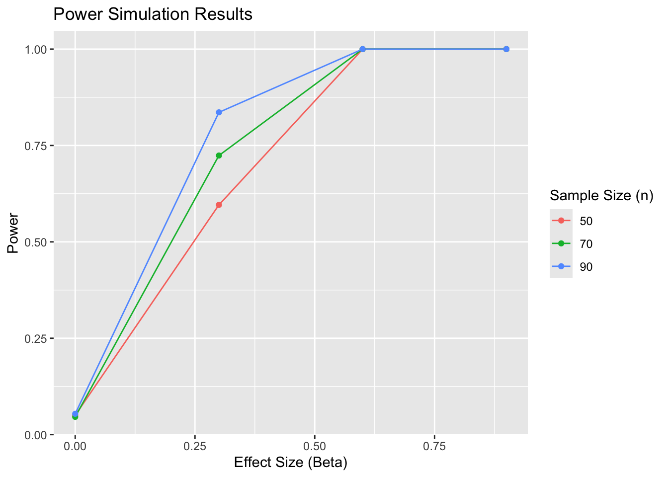
So power is roughly the same as alpha (0.05), that’s good. Can generate power curves for varying n and beta
From this we can see the basic framework of a power simulation. Now we have to adapt it for factorial MR in cancer survival.
That means the dgm function needs to generate
genotype
proteomic
time to event
And the estimation function needs to run a factorial MR analysis on time to event
For the time to event part, we can simulate the data using the simsurv package. First generate the protein levels and their interaction
n <-10000g1 <-rbinom(n, 2, 0.3) # genotype for protein 1g2 <-rbinom(n, 2, 0.4) # genotype for protein 2u <-rnorm(n) # unmeasured confounderpred1 <-0.5* g1 +0.3* upred2 <-0.5* g2 +0.3* ucovars <-tibble(protein1 = pred1 +rnorm(n, sd =sqrt(1-var(pred1))),protein2 = pred2 +rnorm(n, sd =sqrt(1-var(pred2))),interaction = protein1 * protein2)# we'll need the shape and scale parameters for the Weibull distribution - you can get these from fitting a Weibull model to real data. e.g.lambdas <-1.5gammas <-0.01# And now we select some hypothesised betas for the proteins and their interactionbetas <-c(protein1 =0.3, protein2 =0.4, interaction =0.2)# Finally we need a max time for the simulation. This will introduce right-censoring e.g.maxt <-5simdata <-simsurv(lambdas = lambdas,gammas = gammas,betas = betas,x = covars,maxt = maxt)head(simdata)
For estimation part, if this was just an observational analysis we could use the survival package to fit a Cox proportional hazards model using the survival package. For example:
cox_model <-coxph(Surv(eventtime, status) ~ protein1 + protein2 + interaction, data =merge(covars, simdata, by ="row.names"))summary(cox_model)
So overall the power simulation framework will be similar to the linear regression example, but with a more complex dgm and estimation function.
dgm <-function(n =1000, freq1, freq2, rsq_g1p1, rsq_g2p2, beta_p1, beta_p2, beta_interaction, beta_u, lambdas, gammas, maxt) { g1 <-rbinom(n, 2, freq1) # genotype for protein 1 g2 <-rbinom(n, 2, freq2) # genotype for protein 2 u <-rnorm(n) # unmeasured confounder that induces correlation between protein 1 and 2 pred1 <-scale(g1) * rsq_g1p1 + beta_u * u pred2 <-scale(g2) * rsq_g2p2 + beta_u * u covars <-tibble(protein1 = pred1 +rnorm(n, sd =sqrt(1-var(pred1))),protein2 = pred2 +rnorm(n, sd =sqrt(1-var(pred2))),interaction = protein1 * protein2) betas <-c(protein1 = beta_p1, protein2 = beta_p2, interaction = beta_interaction) simdata <-simsurv(lambdas = lambdas,gammas = gammas,betas = betas,x = covars,maxt = maxt) d <-cbind(covars, simdata, g1, g2) %>%as_tibble()return(d)}
Note that there’s quite a lot of parameters that could vary in the dgm, but you could fix many of those cos you know what they are in the real data (e.g. n, freq1, freq2, rsq, beta_p1, beta_p2, lambdas, gammas, maxt values). So you’d end up varying the beta_interaction values and beta_u values only