Background
If \(Y\) includes related samples, why is it beneficial to adjust for PRS, or to take residuals from the LMM, in order to perform regression without the issue of non-independence?
Data generating model:
\[
Y = \sigma^2_g K + \sigma^2_e I
\]
where \(K\) is the kinship matrix and \(I\) is the identity matrix.
The PRS is an estimate of \(\sigma^2_g K\) , which means the residual of \(Y\) will reduce to the uncorrelated term \(\sigma^2_e I\) . However it’s not clear how well the PRS method will work if it’s an imperfect measure of \(\sigma^2_g K\) , and it also is a question as to whether correcting for the complete or incomplete PRS will help with vQTL estimates.
Create y from lots of gs
duplicate some values of y
regress x on y
predict y from gs and adjust for prediction
regression x on y resid
Attaching package: 'dplyr'
The following objects are masked from 'package:stats':

    filter, lag
The following objects are masked from 'package:base':

    intersect, setdiff, setequal, union
library (ggplot2)<- 20 <- 50 <- group_size * ngroup<- 100 <- matrix (rbinom (group_size * p, 2 , 0.5 ), group_size, p)<- rnorm (p)<- rep (scale (g %*% betas), each= ngroup)<- rnorm (n)<- (prs + e) %>% scale %>% drop
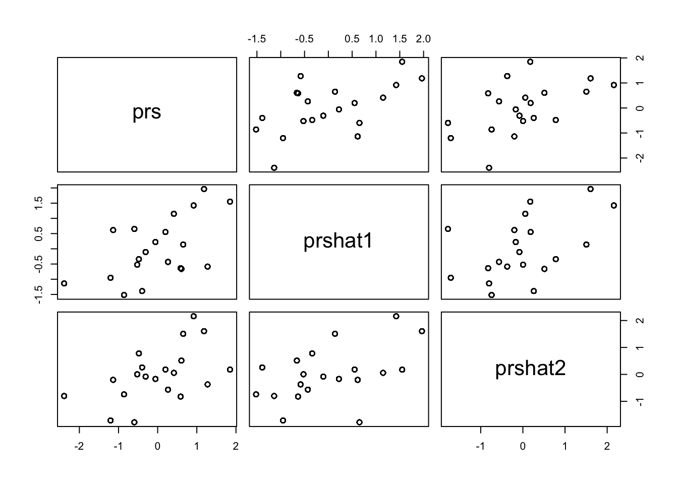
Now generate estimates of the PRS.
Betas are imperfectly estimates
Only some Betas are included
<- rnorm (p, betas)<- rep (scale (g %*% betahat), each= ngroup)<- rep (scale (g[,1 : (p/ 2 )] %*% betas[1 : (p/ 2 )]), each= ngroup)
pairs (cbind (prs, prshat1, prshat2))
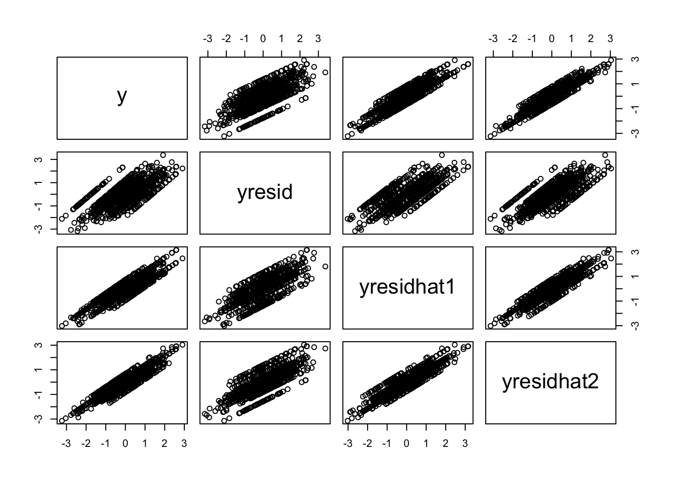
Generate residuals
<- residuals (lm (y ~ prs)) %>% scale %>% drop<- residuals (lm (y ~ prshat1)) %>% scale %>% drop<- residuals (lm (y ~ prshat2)) %>% scale %>% droppairs (cbind (y, yresid, yresidhat1, yresidhat2))
Function for vQTL estimation
<- function (g, y) {<- tapply (y, g, median, na.rm= T) <- abs (y - y.i[g+ 1 ])summary (lm (z.ij ~ g))$ coef %>% as_tibble () %>% slice (2 ) %>% mutate (method= "drm" )<- function (g, y) {summary (lm (y ~ g))$ coef %>% as_tibble () %>% slice (2 ) %>% mutate (method= "add" )
Run simulations
Null SNP
Strong relatedness
Y is adjusted for different levels of PRS
Additive (add) and vQTL models (drm)
1000 replicates
<- expand.grid (y_options = c ("y" , "yresid" , "yresidhat1" , "yresidhat2" ),method_options = c ("drm" , "add" ),stringsAsFactors= FALSE <- lapply (1 : 1000 , \(i) {<- rep (rbinom (group_size, 2 , 0.5 ), each = ngroup)lapply (1 : nrow (params), \(j) {<- get (params$ method_options[j])<- get (params$ y_options[j])m (SNP, yo) %>% mutate (what = params$ y_options[j])%>% bind_rows ()%>% bind_rows ()names (sims) <- c ("b" , "se" , "tval" , "pval" , "method" , "what" )
# A tibble: 7,984 × 6
          b     se   tval     pval method what
      <dbl>  <dbl>  <dbl>    <dbl> <chr>  <chr>
 1  0.0695  0.0216  3.22  1.31e- 3 drm    y
 2  0.0112  0.0222  0.503 6.15e- 1 drm    yresid
 3  0.00680 0.0214  0.318 7.51e- 1 drm    yresidhat1
 4  0.0108  0.0212  0.511 6.10e- 1 drm    yresidhat2
 5 -0.0627  0.0365 -1.72  8.63e- 2 add    y
 6 -0.0393  0.0366 -1.07  2.83e- 1 add    yresid
 7 -0.224   0.0359 -6.23  6.70e-10 add    yresidhat1
 8 -0.281   0.0355 -7.91  6.70e-15 add    yresidhat2
 9  0.162   0.0308  5.26  1.72e- 7 drm    y
10  0.0141  0.0327  0.432 6.66e- 1 drm    yresid
# ℹ 7,974 more rows
Mean absolute values from the simulations
%>% group_by (method, what) %>% summarise (b= mean (abs (b)), se= mean (se), pval= mean (pval), tval= mean (abs (tval)))
`summarise()` has grouped output by 'method'. You can override using the
`.groups` argument.
# A tibble: 8 × 6
# Groups:   method [2]
  method what            b     se  pval  tval
  <chr>  <chr>       <dbl>  <dbl> <dbl> <dbl>
1 add    y          0.204  0.0460 0.116 4.53
2 add    yresid     0.0485 0.0467 0.415 1.04
3 add    yresidhat1 0.183  0.0462 0.129 4.03
4 add    yresidhat2 0.194  0.0461 0.125 4.28
5 drm    y          0.0778 0.0273 0.174 2.88
6 drm    yresid     0.0179 0.0283 0.568 0.630
7 drm    yresidhat1 0.0597 0.0271 0.220 2.21
8 drm    yresidhat2 0.0714 0.0274 0.186 2.62
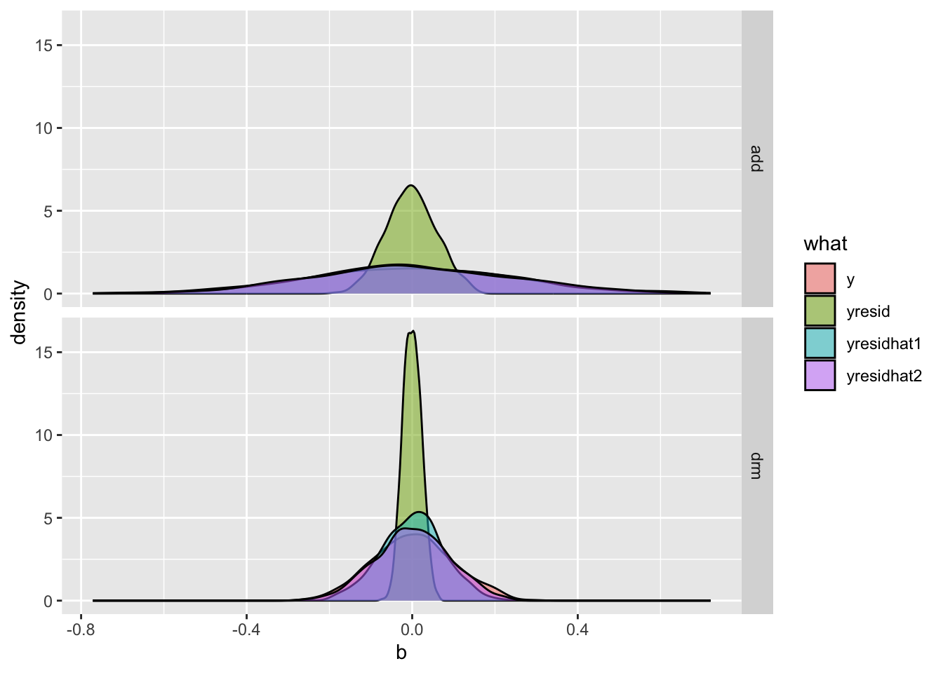
Look at difference in betas
ggplot (sims, aes (x= b)) + geom_density (aes (fill= what), alpha= 0.5 ) + facet_grid (method ~ .)
Summary
Full adjustment for PRS will remove type 1 error for both vQTLs and additive effects
The standard error is not affected by the adjustment
The betas are attenuated when PRS is more effectively captured
R version 4.5.1 (2025-06-13)
Platform: aarch64-apple-darwin20
Running under: macOS Sonoma 14.6.1

Matrix products: default
BLAS:   /Library/Frameworks/R.framework/Versions/4.5-arm64/Resources/lib/libRblas.0.dylib
LAPACK: /Library/Frameworks/R.framework/Versions/4.5-arm64/Resources/lib/libRlapack.dylib;  LAPACK version 3.12.1

locale:
[1] en_US.UTF-8/en_US.UTF-8/en_US.UTF-8/C/en_US.UTF-8/en_US.UTF-8

time zone: Europe/London
tzcode source: internal

attached base packages:
[1] stats     graphics  grDevices utils     datasets  methods   base

other attached packages:
[1] ggplot2_3.5.2 dplyr_1.1.4

loaded via a namespace (and not attached):
 [1] vctrs_0.6.5        cli_3.6.5          knitr_1.50         rlang_1.1.6
 [5] xfun_0.52          generics_0.1.4     jsonlite_2.0.0     labeling_0.4.3
 [9] glue_1.8.0         htmltools_0.5.8.1  scales_1.4.0       rmarkdown_2.29
[13] grid_4.5.1         evaluate_1.0.4     tibble_3.3.0       fastmap_1.2.0
[17] yaml_2.3.10        lifecycle_1.0.4    compiler_4.5.1     RColorBrewer_1.1-3
[21] htmlwidgets_1.6.4  pkgconfig_2.0.3    farver_2.1.2       digest_0.6.37
[25] R6_2.6.1           utf8_1.2.6         tidyselect_1.2.1   pillar_1.11.0
[29] magrittr_2.0.3     withr_3.0.2        tools_4.5.1        gtable_0.3.6