Background
Suppose this is the model:
G1 -> childhood BMI
         |
         V
G2 -> adulthood BMI -> BC
If the childhood BMI GWAS and the adulthood GWAS are different sample sizes, how does this influence the MVMR performance?
Simulations
library (simulateGP)library (dplyr)
Attaching package: 'dplyr'
The following objects are masked from 'package:stats':

    filter, lag
The following objects are masked from 'package:base':

    intersect, setdiff, setequal, union
Loading required package: future
library (ggplot2)<- function (ss1, ss2, ssout) {<- c (subset (ss1, pval < 5e-8 )$ snp,subset (ss2, pval < 5e-8 )$ snp%>% unique<- subset (ss1, snp %in% snplist)$ bhat<- subset (ss2, snp %in% snplist)$ bhat<- subset (ssout, snp %in% snplist)$ bhat<- subset (ssout, snp %in% snplist)$ se<- summary (lm (bout ~ 0 + b1 + b2, weight= 1 / seout^ 2 ))$ coef %>% as_tibble ()names (mod) <- c ("b" , "se" , "tval" , "pval" )<- mutate (mod, trait= c ("1" , "2" ), ninst = c (sum (ss1$ pval < 5e-8 ), sum (ss2$ pval < 5e-8 )))return (mod)<- function (nsnp, h2_1, h2_2, Pi_1, Pi_2, b_12, nid1, nid2, nid3, b_1o, b_2o, rep= NULL , gxe= NULL ) {<- arbitrary_map (runif (nsnp, 0.01 , 0.99 ))<- generate_gwas_params (map= map, h2= h2_1, S= - 0.1 , Pi= Pi_1)<- generate_gwas_params (map= map, h2= h2_2, S= - 0.1 , Pi= Pi_2)$ beta <- params2$ beta + params1$ beta * b_12<- generate_gwas_ss (params1, nid= nid1)<- generate_gwas_ss (params2, nid= nid2)<- params2$ beta <- params1$ beta * b_1o + params2$ beta * b_2o<- generate_gwas_ss (params3, nid= 300000 )return (list (ss1, ss2, ssout))
Example
<- generate_data (nsnp = 1000000 ,h2_1 = 0.3 ,h2_2 = 0.3 ,Pi_1 = 0.02 ,Pi_2 = 0.02 ,b_12 = 0.8 ,nid1 = 220000 ,nid2 = 220000 ,nid3 = 300000 ,b_1o = 0 ,b_2o = - 0.5 str (dat)
List of 3
 $ : tibble [1,000,000 × 11] (S3: tbl_df/tbl/data.frame)
  ..$ snp : int [1:1000000] 1 2 3 4 5 6 7 8 9 10 ...
  ..$ chr : num [1:1000000] 99 99 99 99 99 99 99 99 99 99 ...
  ..$ pos : int [1:1000000] 1 2 3 4 5 6 7 8 9 10 ...
  ..$ ea  : chr [1:1000000] "1" "1" "1" "1" ...
  ..$ oa  : chr [1:1000000] "2" "2" "2" "2" ...
  ..$ af  : num [1:1000000] 0.325 0.329 0.491 0.247 0.419 ...
  ..$ se  : num [1:1000000] 0.00322 0.00321 0.00302 0.00349 0.00306 ...
  ..$ bhat: num [1:1000000] 1.04e-03 4.80e-05 1.01e-03 6.61e-04 6.47e-05 ...
  ..$ fval: num [1:1000000] 0.104388 0.000223 0.113153 0.03582 0.000448 ...
  ..$ n   : num [1:1000000] 220000 220000 220000 220000 220000 220000 220000 220000 220000 220000 ...
  ..$ pval: num [1:1000000] 0.747 0.988 0.737 0.85 0.983 ...
 $ : tibble [1,000,000 × 11] (S3: tbl_df/tbl/data.frame)
  ..$ snp : int [1:1000000] 1 2 3 4 5 6 7 8 9 10 ...
  ..$ chr : num [1:1000000] 99 99 99 99 99 99 99 99 99 99 ...
  ..$ pos : int [1:1000000] 1 2 3 4 5 6 7 8 9 10 ...
  ..$ ea  : chr [1:1000000] "1" "1" "1" "1" ...
  ..$ oa  : chr [1:1000000] "2" "2" "2" "2" ...
  ..$ af  : num [1:1000000] 0.325 0.329 0.491 0.247 0.419 ...
  ..$ se  : num [1:1000000] 0.00322 0.00321 0.00302 0.00349 0.00306 ...
  ..$ bhat: num [1:1000000] -1.87e-04 -1.81e-04 3.02e-04 2.84e-05 1.54e-03 ...
  ..$ fval: num [1:1000000] 3.37e-03 3.18e-03 1.00e-02 6.62e-05 2.53e-01 ...
  ..$ n   : num [1:1000000] 220000 220000 220000 220000 220000 220000 220000 220000 220000 220000 ...
  ..$ pval: num [1:1000000] 0.954 0.955 0.92 0.994 0.615 ...
 $ : tibble [1,000,000 × 11] (S3: tbl_df/tbl/data.frame)
  ..$ snp : int [1:1000000] 1 2 3 4 5 6 7 8 9 10 ...
  ..$ chr : num [1:1000000] 99 99 99 99 99 99 99 99 99 99 ...
  ..$ pos : int [1:1000000] 1 2 3 4 5 6 7 8 9 10 ...
  ..$ ea  : chr [1:1000000] "1" "1" "1" "1" ...
  ..$ oa  : chr [1:1000000] "2" "2" "2" "2" ...
  ..$ af  : num [1:1000000] 0.325 0.329 0.491 0.247 0.419 ...
  ..$ se  : num [1:1000000] 0.00276 0.00275 0.00258 0.00299 0.00262 ...
  ..$ bhat: num [1:1000000] 0.00207 0.000835 0.003009 0.001452 -0.003564 ...
  ..$ fval: num [1:1000000] 0.5643 0.0923 1.3579 0.2355 1.8554 ...
  ..$ n   : num [1:1000000] 3e+05 3e+05 3e+05 3e+05 3e+05 3e+05 3e+05 3e+05 3e+05 3e+05 ...
  ..$ pval: num [1:1000000] 0.453 0.761 0.244 0.628 0.173 ...
do_mvmr (dat[[1 ]], dat[[2 ]], dat[[3 ]])
# A tibble: 2 × 6
        b     se   tval      pval trait ninst
    <dbl>  <dbl>  <dbl>     <dbl> <chr> <int>
1 -0.0651 0.0128  -5.07 5.67e-  7 1       230
2 -0.390  0.0110 -35.6  1.16e-136 2       283
Here, the power is the same for the two exposures, and we get an appropriate result of exposure 2 having the causal influence.
Analysis
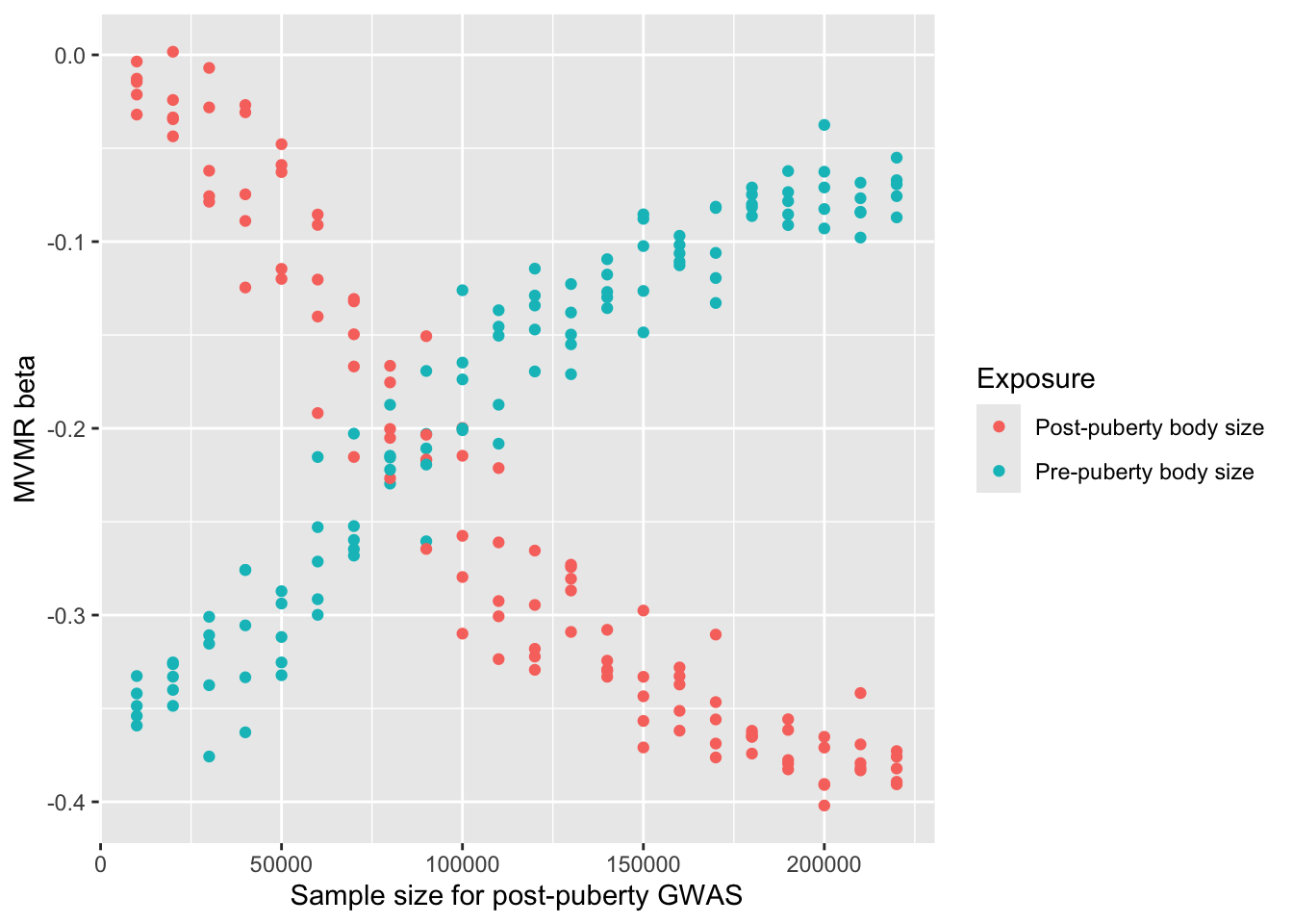
Run simulations with different sample sizes for the exposure 2 (the real causal exposure)
<- expand.grid (nsnp = 1000000 ,h2_1 = 0.3 ,h2_2 = 0.1 ,Pi_1 = 0.02 ,Pi_2 = 0.005 ,b_12 = 0.9 ,gxe = 0 ,nid1 = 220000 ,nid2 = seq (10000 , 220000 , by= 10000 ),nid3 = 300000 ,b_1o = 0 ,b_2o = - 0.5 ,rep = 1 : 5 <- function (...) {<- list (...)<- do.call (generate_data, l)<- do_mvmr (dat[[1 ]], dat[[2 ]], dat[[3 ]])<- bind_cols (res, as_tibble (l))plan (multicore, workers= 6 )<- future_pmap (params, run_sim, .options= furrr_options (seed= TRUE )) %>% bind_rows ()
%>% mutate (trait = case_when (trait == 1 ~ "Pre-puberty body size" , trait == 2 ~ "Post-puberty body size" )%>% ggplot (aes (x= nid2, y= b, colour= as.factor (trait))) + geom_point () + labs (x= "Sample size for post-puberty GWAS" , y= "MVMR beta" , colour= "Exposure" )
Summary
This is probably well known, but when X2 is causal but has low power, X1 will appear to be the causal factor
Empirically we see the below, so this power issue is not the whole story.
childhood (high power)
  |
  v
adolescent (low power) -> BC

- adolescent attenuates when power is low


adolescent (low power) -> BC
  |
  v
adult (high power)

- adult attenuates even though power is high
R version 4.5.1 (2025-06-13)
Platform: aarch64-apple-darwin20
Running under: macOS Sonoma 14.6.1

Matrix products: default
BLAS:   /Library/Frameworks/R.framework/Versions/4.5-arm64/Resources/lib/libRblas.0.dylib
LAPACK: /Library/Frameworks/R.framework/Versions/4.5-arm64/Resources/lib/libRlapack.dylib;  LAPACK version 3.12.1

locale:
[1] en_US.UTF-8/en_US.UTF-8/en_US.UTF-8/C/en_US.UTF-8/en_US.UTF-8

time zone: Europe/London
tzcode source: internal

attached base packages:
[1] stats     graphics  grDevices utils     datasets  methods   base

other attached packages:
[1] ggplot2_3.5.2    furrr_0.3.1      future_1.49.0    dplyr_1.1.4
[5] simulateGP_0.1.3

loaded via a namespace (and not attached):
 [1] gtable_0.3.6       jsonlite_2.0.0     compiler_4.5.1     tidyselect_1.2.1
 [5] parallel_4.5.1     globals_0.18.0     scales_1.4.0       yaml_2.3.10
 [9] fastmap_1.2.0      R6_2.6.1           labeling_0.4.3     generics_0.1.4
[13] knitr_1.50         htmlwidgets_1.6.4  tibble_3.3.0       pillar_1.11.0
[17] RColorBrewer_1.1-3 rlang_1.1.6        utf8_1.2.6         xfun_0.52
[21] cli_3.6.5          withr_3.0.2        magrittr_2.0.3     digest_0.6.37
[25] grid_4.5.1         lifecycle_1.0.4    vctrs_0.6.5        evaluate_1.0.4
[29] glue_1.8.0         farver_2.1.2       listenv_0.9.1      codetools_0.2-20
[33] parallelly_1.44.0  rmarkdown_2.29     purrr_1.1.0        tools_4.5.1
[37] pkgconfig_2.0.3    htmltools_0.5.8.1