Background
Does meta analysis with very small samples lead to bias?
Simulate a regression
Split the data into different size groups and meta analyse the groups
Compare the meta-analysis results to the full analysis
Does smaller group size lead to bias?
Attaching package: 'dplyr'
The following objects are masked from 'package:stats':

    filter, lag
The following objects are masked from 'package:base':

    intersect, setdiff, setequal, union
library (ggplot2)library (tidyr)<- function (betas, ses) {<- 1 / ses^ 2 <- sum (weights * betas) / sum (weights)<- 1 / sqrt (sum (weights))return (c (beta, se))
<- function (y, x) {<- is.finite (y) & is.finite (x)<- sum (index)<- y[index]<- x[index]<- var (x)<- stats:: cov (y, x) / vx<- mean (y) - bhat * mean (x)# fitted <- ahat + x * bhat # residuals <- y - fitted # SSR <- sum((residuals - mean(residuals))^2) # SSF <- sum((fitted - mean(fitted))^2) <- (bhat * vx)^ 2 / (vx * var (y))<- rsq * (n-2 ) / (1 - rsq)<- sqrt (fval)<- abs (bhat / tval)# Fval <- (SSF) / (SSR/(n-2)) # pval <- pf(Fval, 1, n-2, lowe=F) # p <- stats::pf(fval, 1, n-2, lower.tail=FALSE) return (list (ahat= ahat, bhat= bhat, se= se, fval= fval, n= n<- function (n, nbreak, beta, af) {<- rbinom (n, 2 , af)<- g * beta + rnorm (n)<- summary (lm (y ~ g))<- cut (1 : n, breaks= nbreak)<- lapply (levels (breaks), \(l) {<- y[breaks == l]<- g[breaks == l]if (length (unique (g)) == 1 ) return (NULL )<- fast_assoc (y, g)tibble (beta = a$ bhat,se = a$ se%>% bind_rows ()<- ivw (r$ beta, r$ se)tibble (n= n, nbreak= nbreak, beta= beta, af= af,bhat= c (full$ coefficients[2 , 1 ], meta[1 ]),se= c (full$ coefficients[2 , 2 ], meta[2 ]),what= c ("full" , "meta" )sim (10000 , 1000 , 0.2 , 0.5 )
# A tibble: 2 × 7
      n nbreak  beta    af  bhat     se what
  <dbl>  <dbl> <dbl> <dbl> <dbl>  <dbl> <chr>
1 10000   1000   0.2   0.5 0.243 0.0143 full
2 10000   1000   0.2   0.5 0.243 0.0134 meta
<- expand.grid (n = 10000 ,nbreak = c (10 , 100 , 1000 ),beta = c (0 , 0.2 ),af = c (0.1 , 0.5 ),nsim = 1 : 30 dim (param)
<- lapply (1 : nrow (param), \(i) {sim (param$ n[i], param$ nbreak[i], param$ beta[i], param$ af[i]) %>% mutate (sim= param$ nsim[i])%>% bind_rows ()
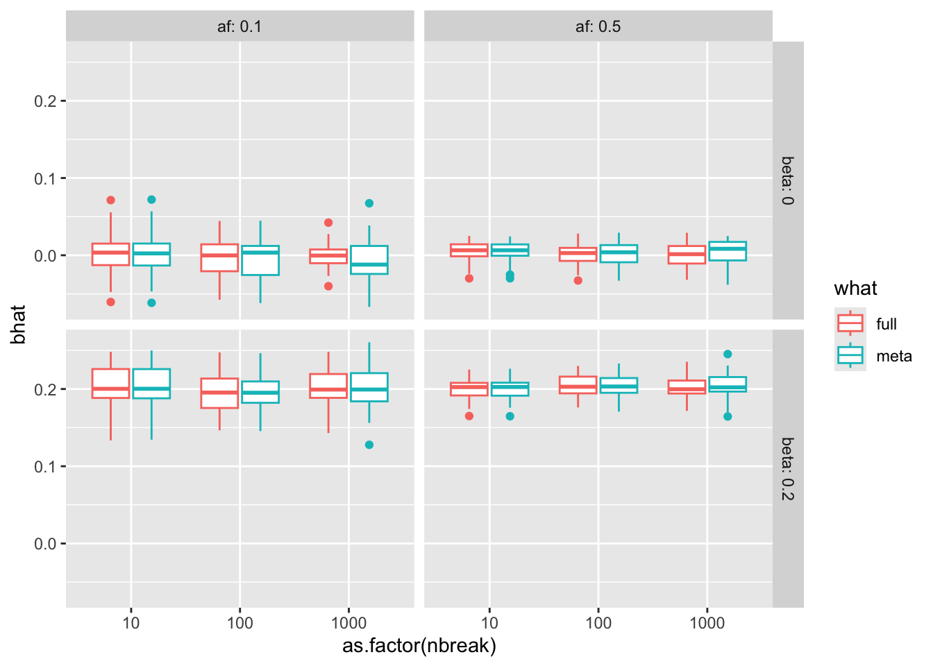
ggplot (res, aes (x= as.factor (nbreak), y= bhat, color= what)) + geom_boxplot () + facet_grid (beta ~ af, labeller= label_both)
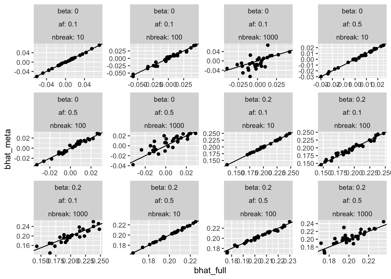
<- pivot_wider (res, names_from= what, values_from= c (bhat, se))ggplot (resw, aes (x= bhat_full, y= bhat_meta)) + geom_point () + facet_wrap (~ beta + af + nbreak, scale= "free" , labeller= label_both) + geom_abline (slope= 1 , intercept= 0 )
Try again with just continuous data
<- function (n, nbreak, beta) {<- rnorm (n)<- g * beta + rnorm (n)<- summary (lm (y ~ g))<- cut (1 : n, breaks= nbreak)<- lapply (levels (breaks), \(l) {<- y[breaks == l]<- g[breaks == l]if (length (unique (g)) == 1 ) return (NULL )<- fast_assoc (y, g)tibble (beta = a$ bhat,se = a$ se%>% bind_rows ()<- ivw (r$ beta, r$ se)tibble (n= n, nbreak= nbreak, beta= beta,bhat= c (full$ coefficients[2 , 1 ], meta[1 ]),se= c (full$ coefficients[2 , 2 ], meta[2 ]),what= c ("full" , "meta" )sim2 (10000 , 1000 , 0.2 )
# A tibble: 2 × 6
      n nbreak  beta  bhat      se what
  <dbl>  <dbl> <dbl> <dbl>   <dbl> <chr>
1 10000   1000   0.2 0.196 0.00999 full
2 10000   1000   0.2 0.192 0.00914 meta
# A tibble: 2 × 6
      n nbreak  beta  bhat      se what
  <dbl>  <dbl> <dbl> <dbl>   <dbl> <chr>
1 10000    100   0.2 0.195 0.00999 full
2 10000    100   0.2 0.196 0.00995 meta
# A tibble: 2 × 6
      n nbreak  beta  bhat     se what
  <dbl>  <dbl> <dbl> <dbl>  <dbl> <chr>
1 10000     10   0.2 0.202 0.0100 full
2 10000     10   0.2 0.202 0.0100 meta
<- expand.grid (n = 10000 ,nbreak = c (10 , 100 , 1000 ),beta = c (0 , 0.2 ),nsim = 1 : 100 dim (param2)
<- lapply (1 : nrow (param2), \(i) {sim2 (param2$ n[i], param2$ nbreak[i], param2$ beta[i]) %>% mutate (sim= param2$ nsim[i])%>% bind_rows ()
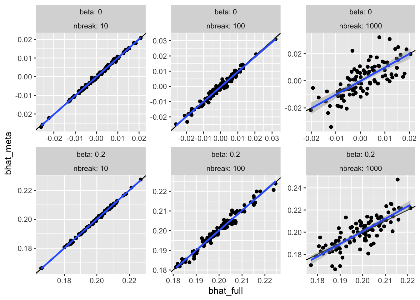
<- pivot_wider (res2, names_from= what, values_from= c (bhat, se))ggplot (resw, aes (x= bhat_full, y= bhat_meta)) + geom_point () + facet_wrap (~ beta + nbreak, scale= "free" , labeller= label_both) + geom_abline (slope= 1 , intercept= 0 ) + geom_smooth (method= "lm" )
`geom_smooth()` using formula = 'y ~ x'
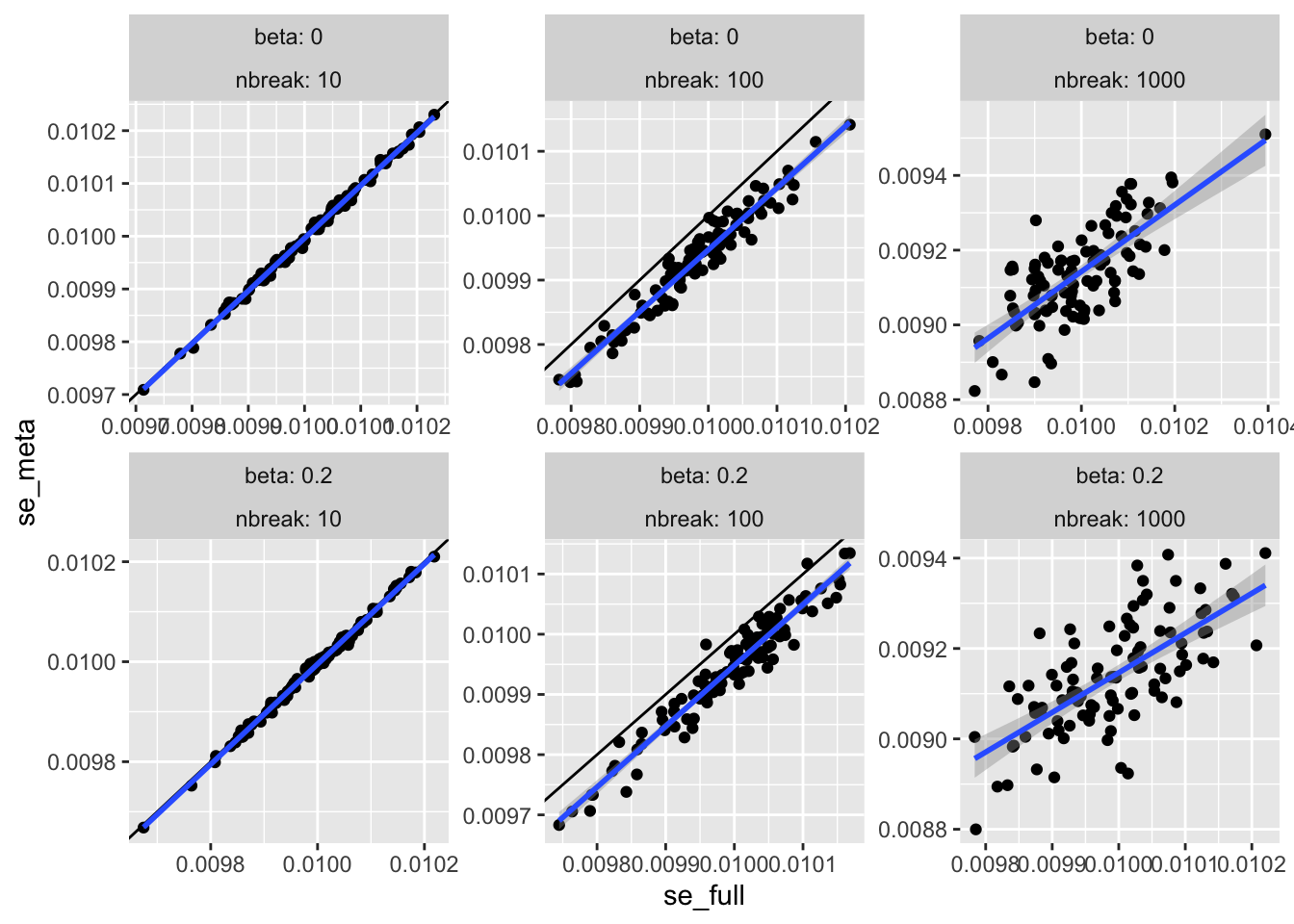
ggplot (resw, aes (x= se_full, y= se_meta)) + geom_point () + facet_wrap (~ beta + nbreak, scale= "free" , labeller= label_both) + geom_abline (slope= 1 , intercept= 0 ) + geom_smooth (method= "lm" )
`geom_smooth()` using formula = 'y ~ x'
%>% mutate (pval = pnorm (abs (bhat)/ se, low= F)) %>% filter (beta == 0 ) %>% group_by (nbreak, what) %>% summarise (power = sum (pval < 0.05 )/ n (), n= n ())
`summarise()` has grouped output by 'nbreak'. You can override using the
`.groups` argument.
# A tibble: 6 × 4
# Groups:   nbreak [3]
  nbreak what  power     n
   <dbl> <chr> <dbl> <int>
1     10 full   0.06   100
2     10 meta   0.06   100
3    100 full   0.1    100
4    100 meta   0.08   100
5   1000 full   0.07   100
6   1000 meta   0.21   100
Simulate one small study
<- function (n, prop, beta, af) {<- rbinom (n, 2 , af)<- g * beta + rnorm (n)<- 1 : (n* prop)<- (1 : n)[- s1]<- 1 : n<- lapply (list (s1, s2, s3), \(s) {<- y[s]<- g[s]if (length (unique (g)) == 1 ) return (NULL )<- fast_assoc (y, g)tibble (bhat = a$ bhat,se = a$ se,ns = length (y)%>% bind_rows () %>% mutate (what= c ("p" , "q" , "full" ))<- ivw (r$ bhat[1 : 2 ], r$ se[1 : 2 ])<- bind_rows (r, tibble (bhat = meta[1 ], se = meta[2 ], ns = n, what= "meta" )) %>% mutate (n= n, prop= prop, beta= beta, af= af)return (r)sim3 (10000 , 0.01 , 0.2 , 0.5 )
# A tibble: 4 × 8
   bhat     se    ns what      n  prop  beta    af
  <dbl>  <dbl> <dbl> <chr> <dbl> <dbl> <dbl> <dbl>
1 0.153 0.147    100 p     10000  0.01   0.2   0.5
2 0.205 0.0144  9900 q     10000  0.01   0.2   0.5
3 0.204 0.0143 10000 full  10000  0.01   0.2   0.5
4 0.204 0.0143 10000 meta  10000  0.01   0.2   0.5
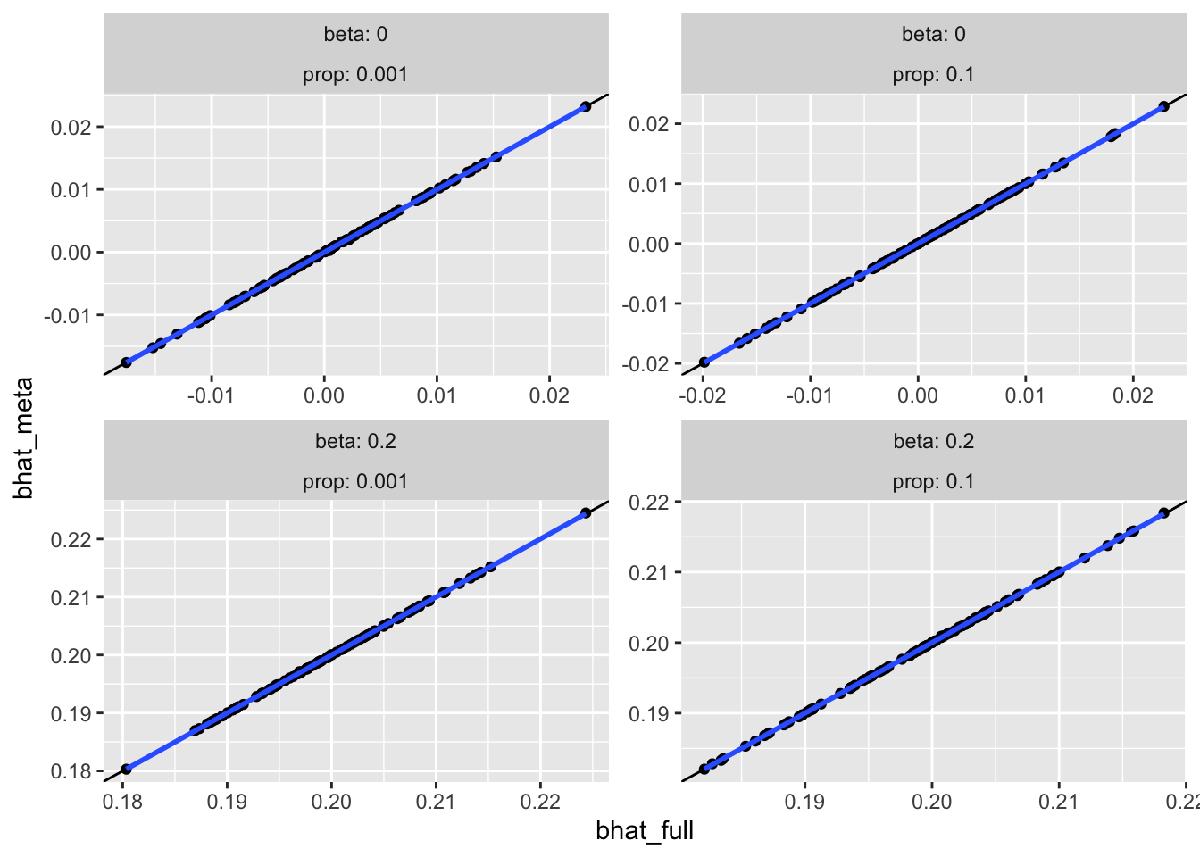
<- expand.grid (n = 100000 ,prop = c (0.1 , 0.001 ),beta = c (0 , 0.2 ),af = c (0.1 ),nsim = 1 : 100 dim (param3)<- lapply (1 : nrow (param3), \(i) {sim3 (param3$ n[i], param3$ prop[i], param3$ beta[i], param3$ af[i]) %>% mutate (sim= param3$ nsim[i])%>% bind_rows ()<- res3 %>% filter (what %in% c ("full" , "meta" )) %>% pivot_wider (names_from= what, values_from= c (bhat, se))ggplot (resw, aes (x= bhat_full, y= bhat_meta)) + geom_point () + facet_wrap (~ beta + prop, scale= "free" , labeller= label_both) + geom_abline (slope= 1 , intercept= 0 ) + geom_smooth (method= "lm" )
`geom_smooth()` using formula = 'y ~ x'
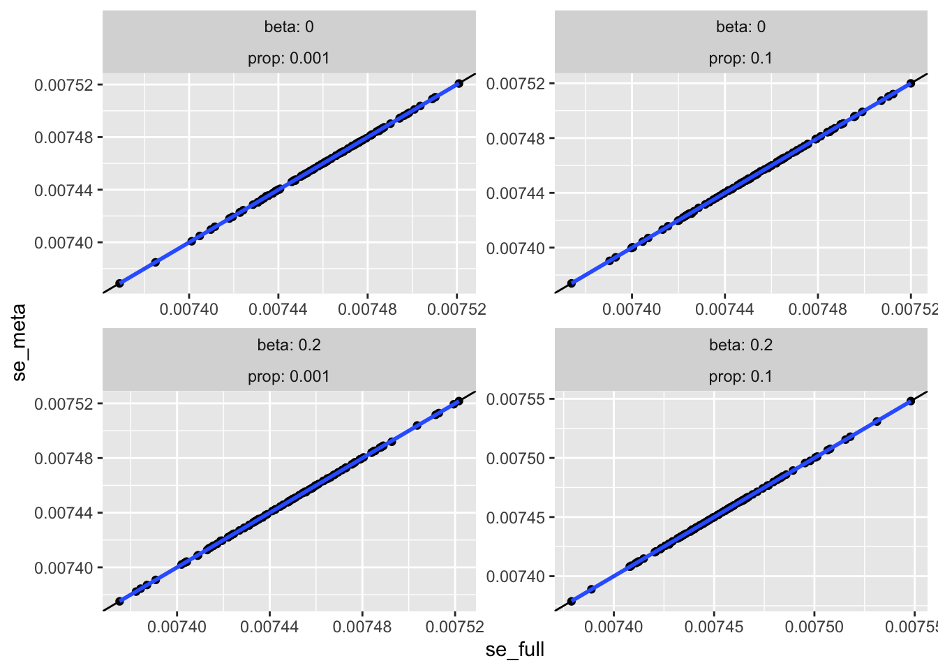
ggplot (resw, aes (x= se_full, y= se_meta)) + geom_point () + facet_wrap (~ beta + prop, scale= "free" , labeller= label_both) + geom_abline (slope= 1 , intercept= 0 ) + geom_smooth (method= "lm" )
`geom_smooth()` using formula = 'y ~ x'
Summary
No bias
For many small studies, the effects are not identical and become more noisy as the sample size decreases.
For many small studies, the standard error is under estimated for the meta analysis as the sample sizes decrease, which leads to slight elevation of type 1 error.
For a single small study there is negligible impact on bias or type 1 error.
R version 4.4.1 (2024-06-14)
Platform: aarch64-apple-darwin20
Running under: macOS Sonoma 14.6.1

Matrix products: default
BLAS:   /Library/Frameworks/R.framework/Versions/4.4-arm64/Resources/lib/libRblas.0.dylib
LAPACK: /Library/Frameworks/R.framework/Versions/4.4-arm64/Resources/lib/libRlapack.dylib;  LAPACK version 3.12.0

locale:
[1] en_US.UTF-8/en_US.UTF-8/en_US.UTF-8/C/en_US.UTF-8/en_US.UTF-8

time zone: Europe/London
tzcode source: internal

attached base packages:
[1] stats     graphics  grDevices utils     datasets  methods   base

other attached packages:
[1] tidyr_1.3.1   ggplot2_3.5.1 dplyr_1.1.4

loaded via a namespace (and not attached):
 [1] Matrix_1.7-0      gtable_0.3.5      jsonlite_1.8.8    compiler_4.4.1
 [5] tidyselect_1.2.1  splines_4.4.1     scales_1.3.0      yaml_2.3.8
 [9] fastmap_1.2.0     lattice_0.22-6    R6_2.5.1          labeling_0.4.3
[13] generics_0.1.3    knitr_1.47        htmlwidgets_1.6.4 tibble_3.2.1
[17] munsell_0.5.1     pillar_1.9.0      rlang_1.1.3       utf8_1.2.4
[21] xfun_0.44         cli_3.6.2         withr_3.0.0       magrittr_2.0.3
[25] mgcv_1.9-1        digest_0.6.35     grid_4.4.1        lifecycle_1.0.4
[29] nlme_3.1-164      vctrs_0.6.5       evaluate_0.23     glue_1.7.0
[33] farver_2.1.2      fansi_1.0.6       colorspace_2.1-0  rmarkdown_2.27
[37] purrr_1.0.2       tools_4.4.1       pkgconfig_2.0.3   htmltools_0.5.8.1