Evaluating replication rates

Author

Gibran Hemani

Published

February 27, 2024

Background

Taking a set of genetic effects in one study and replicating in another - what is the appropriate way to determine if the effects are consistent?

Simulation

set.seed(100)
library(dplyr)

Attaching package: 'dplyr'
The following objects are masked from 'package:stats':

    filter, lag
The following objects are masked from 'package:base':

    intersect, setdiff, setequal, union
library(ggplot2)

sim <- function(n1, n2, nsnp, nflip=1, afshared=FALSE, bsd=1) {
    # different allele frequencies per study
    af1 <- runif(nsnp, 0.01, 0.99)
    if(afshared) {
        af2 <- af1
    } else {
        af2 <- runif(nsnp, 0.01, 0.99)
    }

    # identifical effect sizes across studies
    b1 <- rnorm(nsnp, sd=bsd)
    b2 <- b1

    # make one of the effects different
    if(nflip > 0) {
        b1[1:nflip] <- b1[1:nflip] * -1
    }

    # Assume variance of trait is the same across studies
    se1 <- 1 / sqrt(2 * af1 * (1-af1) * n1)
    se2 <- 1 / sqrt(2 * af2 * (1-af2) * n2)

    dat <- tibble(
        af1, af2, b1, b2, se1, se2,
        bhat1 = rnorm(nsnp, b1, se1),
        bhat2 = rnorm(nsnp, b2, se2),
        pval1 = 2 * pnorm(-abs(bhat1/se1)),
        pval2 = 2 * pnorm(-abs(bhat2/se2)),
        r21 = b1^2 * af1 * (1-af1) * 2,
        r22 = b2^2 * af2 * (1-af2) * 2,
    )
    return(dat)
}

Plot relationship

Simple trait, a few large effects

dat_simple <- sim(
    n1 = 100000, 
    n2 = 10000, 
    nsnp = 10,
    nflip = 0, 
    afshared = TRUE, 
    bsd = sqrt(0.5)/10
)
ggplot(dat_simple, aes(bhat1, bhat2)) +
geom_point() +
geom_errorbarh(aes(xmax = bhat1 + 1.96*se1, xmin = bhat1 - 1.96*se1)) +
geom_errorbar(aes(ymax = bhat2 + 1.96*se2, ymin = bhat2 - 1.96*se2)) +
geom_abline(intercept=0, slope=1) +
geom_smooth(method="lm")
`geom_smooth()` using formula = 'y ~ x'

Complex trait with many small effects

dat_complex <- sim(
    n1 = 100000, 
    n2 = 10000, 
    nsnp = 1000,
    nflip = 0, 
    afshared = TRUE, 
    bsd = sqrt(0.00008)
)
table(dat_complex$pval1 < 5e-8)

FALSE  TRUE 
  995     5 
ggplot(dat_complex, aes(bhat1, bhat2)) +
geom_point() +
geom_errorbarh(aes(xmax = bhat1 + 1.96*se1, xmin = bhat1 - 1.96*se1)) +
geom_errorbar(aes(ymax = bhat2 + 1.96*se2, ymin = bhat2 - 1.96*se2)) +
geom_abline(intercept=0, slope=1) +
geom_smooth(method="lm")
`geom_smooth()` using formula = 'y ~ x'

Relationship between effect sizes

Expect slope to be about 1 because the betas are the same across the two studies. But differences in power could distort this

Slope in simple trait

summary(lm(bhat2 ~ bhat1, data=dat_simple))

Call:
lm(formula = bhat2 ~ bhat1, data = dat_simple)

Residuals:
      Min        1Q    Median        3Q       Max 
-0.010397 -0.006070 -0.002261  0.002275  0.029045 

Coefficients:
             Estimate Std. Error t value Pr(>|t|)    
(Intercept) -0.003745   0.003811  -0.983    0.355    
bhat1        1.162936   0.104661  11.111 3.84e-06 ***
---
Signif. codes:  0 '***' 0.001 '**' 0.01 '*' 0.05 '.' 0.1 ' ' 1

Residual standard error: 0.01204 on 8 degrees of freedom
Multiple R-squared:  0.9391,    Adjusted R-squared:  0.9315 
F-statistic: 123.5 on 1 and 8 DF,  p-value: 3.845e-06

Slope in complex trait

summary(lm(bhat2 ~ bhat1, data=dat_complex))

Call:
lm(formula = bhat2 ~ bhat1, data = dat_complex)

Residuals:
      Min        1Q    Median        3Q       Max 
-0.112320 -0.012697 -0.000413  0.013574  0.128769 

Coefficients:
              Estimate Std. Error t value Pr(>|t|)    
(Intercept) -0.0001423  0.0007271  -0.196    0.845    
bhat1        0.4467767  0.0646851   6.907 8.81e-12 ***
---
Signif. codes:  0 '***' 0.001 '**' 0.01 '*' 0.05 '.' 0.1 ' ' 1

Residual standard error: 0.02298 on 998 degrees of freedom
Multiple R-squared:  0.04562,   Adjusted R-squared:  0.04466 
F-statistic: 47.71 on 1 and 998 DF,  p-value: 8.807e-12

Replication rate

Expect all significant assocs to replicate. But differences in power could distort this

Replication rate in simple trait is 1

dat_simple %>%
    mutate(disc = pval1 < 5e-8, rep = disc & pval2 < 0.05) %>%
    summarise(ndisc=sum(disc), nrep=sum(rep), rate=nrep/ndisc)
# A tibble: 1 × 3
  ndisc  nrep  rate
  <int> <int> <dbl>
1     4     4     1

Replication rate in complex trait is much lower

dat_complex %>%
    mutate(disc = pval1 < 5e-8, rep = disc & pval2 < 0.05) %>%
    summarise(ndisc=sum(disc), nrep=sum(rep), rate=nrep/ndisc)
# A tibble: 1 × 3
  ndisc  nrep  rate
  <int> <int> <dbl>
1     5     2   0.4

Expected vs observed replication rates

We can calculate the expected number to replicate given the differential power (due to sample size and allele frequency differences across studies), and compare this to the observed number to replicate. If fewer replicate than expected, then this is evidence of heterogeneity in the effect sizes.

#' Estimate expected vs observed replication of effects between discovery and replication datasets
#' 
#' Taken from Okbay et al 2016. Under the assumption that all discovery effects are unbiased, what fraction of associations would replicate in the replication dataset, given the differential power of the discovery and replication datasets.
#' Uses standard error of the replication dataset to account for differences in sample size and distribution of independent variable
#' 
#' @param b_disc Vector of discovery betas
#' @param b_rep Vector of replication betas
#' @param se_disc Vector of discovery standard errors
#' @param se_rep Vector of replication standard errors
#' @param alpha Nominal replication significance threshold
#' 
#' @return List of results
#' - res: aggregate expected replication rate vs observed replication rate
#' - variants: per variant expected replication rates
prop_overlap <- function(b_disc, b_rep, se_disc, se_rep, alpha) {
  p_sign <- pnorm(-abs(b_disc) / se_disc) * pnorm(-abs(b_disc) / se_rep) + ((1 - pnorm(-abs(b_disc) / se_disc)) * (1 - pnorm(-abs(b_disc) / se_rep)))
  p_sig <- pnorm(-abs(b_disc) / se_rep + qnorm(alpha / 2)) + (1 - pnorm(-abs(b_disc) / se_rep - qnorm(alpha / 2)))
  p_rep <- pnorm(abs(b_rep) / se_rep, lower.tail = FALSE)
  res <- tibble::tibble(
    nsnp = length(b_disc),
    metric = c("Sign", "Sign", "P-value", "P-value"),
    datum = c("Expected", "Observed", "Expected", "Observed"),
    value = c(sum(p_sign, na.rm = TRUE), sum(sign(b_disc) == sign(b_rep)), sum(p_sig, na.rm = TRUE), sum(p_rep < alpha, na.rm = TRUE))
  ) %>%
    dplyr::group_by(metric) %>%
      dplyr::do({
        x <- .
        if(.$nsnp[1] > 0) {
          bt <- binom.test(
            x=.$value[.$datum == "Observed"], 
            n=.$nsnp[1], 
            p=.$value[.$datum == "Expected"] / .$nsnp[1]
          )$p.value
          x$pdiff <- bt
        }
        x
      })
  return(list(res = res, variants = dplyr::tibble(sig = p_sig, sign = p_sign, )))
}

Simple trait

with(dat_simple %>% filter(pval1 < 5e-8), prop_overlap(bhat1, bhat2, se1, se2, 0.05))$res
# A tibble: 4 × 5
# Groups:   metric [2]
   nsnp metric  datum    value pdiff
  <int> <chr>   <chr>    <dbl> <dbl>
1     4 P-value Expected  3.34     1
2     4 P-value Observed  4        1
3     4 Sign    Expected  3.99     1
4     4 Sign    Observed  4        1

This shows that we expect all significant discovery associations to replicate, and indeed they do.

Complex trait

with(dat_complex %>% filter(pval1 < 5e-8), prop_overlap(bhat1, bhat2, se1, se2, 0.05))$res
# A tibble: 4 × 5
# Groups:   metric [2]
   nsnp metric  datum    value pdiff
  <int> <chr>   <chr>    <dbl> <dbl>
1     5 P-value Expected  2.35     1
2     5 P-value Observed  2        1
3     5 Sign    Expected  4.85     1
4     5 Sign    Observed  5        1

This shows that we don’t expect all significant discovery associations to replicate, and indeed they don’t, but the rate of observed replication matches the expected rate of replication. The pdiff column is the p-value from a binomial test comparing the observed and expected replication rates, a low p-value indicates that the observed replication rate is substantially different from the expected replication rate.

Heterogeneity

Evaluate if any one particular variant has heterogeneity in effect sizes across the two studies. This is done using Cochrane’s Q statistic, which accounts for difference in power (based on SE) across the studies.

fixed_effects_meta_analysis <- function(beta_vec, se_vec) {
    w <- 1 / se_vec^2
    beta <- sum(beta_vec * w, na.rm=T) / sum(w, na.rm=T)
    se <- sqrt(1 / sum(w, na.rm=T))
    pval <- pnorm(abs(beta / se), lower.tail = FALSE)
    Qj <- w * (beta-beta_vec)^2
    Q <- sum(Qj, na.rm=T)
    Qdf <- sum(!is.na(beta_vec))-1
    if(Qdf == 0) Q <- 0
    Qjpval <- pchisq(Qj, 1, lower.tail=FALSE)
    Qpval <- pchisq(Q, Qdf, lower.tail=FALSE)
    return(list(beta=beta, se=se, pval=pval, Q=Q, Qdf=Qdf, Qpval=Qpval, Qj=Qj, Qjpval=Qjpval))
}

Simple trait, per-variant heterogeneity

het_simple <- lapply(1:nrow(dat_simple), \(i) {
    o <- fixed_effects_meta_analysis(c(dat_simple$bhat1[i], dat_simple$bhat2[i]), c(dat_simple$se1[i], dat_simple$se2[i]))
    tibble(
        SNP = i,
        beta = o$beta,
        se = o$se,
        pval = o$pval,
        Q = o$Q,
        Qdf = o$Qdf,
        Qpval = o$Qpval
    )
}) %>% bind_rows() %>%
    mutate(Qfdr = p.adjust(Qpval, method="fdr"))

het_simple
# A tibble: 10 × 8
     SNP     beta      se     pval       Q   Qdf Qpval  Qfdr
   <int>    <dbl>   <dbl>    <dbl>   <dbl> <dbl> <dbl> <dbl>
 1     1  0.0218  0.00460 1.10e- 6 0.167       1 0.682 0.964
 2     2 -0.0440  0.00485 5.52e-20 0.324       1 0.569 0.964
 3     3  0.0529  0.00429 2.64e-35 0.00438     1 0.947 0.964
 4     4 -0.0689  0.00863 7.30e-16 0.686       1 0.407 0.964
 5     5 -0.0157  0.00427 1.17e- 4 0.213       1 0.645 0.964
 6     6  0.00446 0.00427 1.48e- 1 0.00204     1 0.964 0.964
 7     7  0.0136  0.00539 5.86e- 3 2.09        1 0.148 0.964
 8     8 -0.0133  0.00441 1.24e- 3 0.0443      1 0.833 0.964
 9     9  0.0553  0.00428 1.70e-38 0.115       1 0.734 0.964
10    10  0.00322 0.00559 2.82e- 1 0.170       1 0.680 0.964

Complex trait, per variant heterogeneity

het_complex <- lapply(1:nrow(dat_complex), \(i) {
    o <- fixed_effects_meta_analysis(c(dat_complex$bhat1[i], dat_complex$bhat2[i]), c(dat_complex$se1[i], dat_complex$se2[i]))
    tibble(
        SNP = i,
        beta = o$beta,
        se = o$se,
        pval = o$pval,
        Q = o$Q,
        Qdf = o$Qdf,
        Qpval = o$Qpval
    )
}) %>% bind_rows() %>%
    mutate(Qfdr = p.adjust(Qpval, method="fdr"))

het_complex
# A tibble: 1,000 × 8
     SNP      beta      se    pval      Q   Qdf  Qpval  Qfdr
   <int>     <dbl>   <dbl>   <dbl>  <dbl> <dbl>  <dbl> <dbl>
 1     1 -0.00360  0.00433 0.203   1.10       1 0.295  0.934
 2     2  0.00692  0.00453 0.0632  3.98       1 0.0460 0.867
 3     3 -0.0110   0.00431 0.00536 0.0568     1 0.812  0.980
 4     4  0.0233   0.0106  0.0138  0.0291     1 0.864  0.988
 5     5  0.000229 0.00450 0.480   0.0512     1 0.821  0.981
 6     6  0.000567 0.00440 0.449   0.0778     1 0.780  0.976
 7     7 -0.0112   0.00596 0.0300  0.272      1 0.602  0.942
 8     8 -0.000199 0.00506 0.484   0.440      1 0.507  0.934
 9     9 -0.00530  0.00564 0.174   5.51       1 0.0189 0.767
10    10  0.0129   0.00712 0.0351  0.502      1 0.478  0.934
# ℹ 990 more rows

Try simulating where some of the effects are actually different

dat_dif <- sim(
    n1 = 100000, 
    n2 = 10000, 
    nsnp = 100,
    nflip = 10, 
    afshared = FALSE, 
    bsd = sqrt(0.5)/10
)

Replication rate estimate

prop_overlap(dat_dif$bhat1, dat_dif$bhat2, dat_dif$se1, dat_dif$se2, 0.05)$res
# A tibble: 4 × 5
# Groups:   metric [2]
   nsnp metric  datum    value   pdiff
  <int> <chr>   <chr>    <dbl>   <dbl>
1   100 P-value Expected  60.6 0.838  
2   100 P-value Observed  62   0.838  
3   100 Sign    Expected  92.3 0.00462
4   100 Sign    Observed  84   0.00462

In this situation the effects have the same magnitude (so the p-values should give comparable estimates), but the signs are different for some of the effects. This is reflected in the observed replication rate for the sign, which is lower than the expected replication rate.

Heterogeneity estimate

het_dif <- lapply(1:nrow(dat_dif), \(i) {
    o <- fixed_effects_meta_analysis(c(dat_dif$bhat1[i], dat_dif$bhat2[i]), c(dat_dif$se1[i], dat_dif$se2[i]))
    tibble(
        SNP = i,
        beta = o$beta,
        se = o$se,
        pval = o$pval,
        Q = o$Q,
        Qdf = o$Qdf,
        Qpval = o$Qpval
    )
}) %>% bind_rows() %>%
    mutate(Qfdr = p.adjust(Qpval, method="fdr"))
het_dif %>% filter(Qfdr < 0.05)
# A tibble: 10 × 8
     SNP    beta      se     pval      Q   Qdf    Qpval     Qfdr
   <int>   <dbl>   <dbl>    <dbl>  <dbl> <dbl>    <dbl>    <dbl>
 1     2  0.0721 0.00668 2.11e-27  57.2      1 3.92e-14 1.31e-12
 2     3 -0.0371 0.00744 3.10e- 7  54.5      1 1.56e-13 3.90e-12
 3     4 -0.0635 0.00509 5.09e-36 118.       1 2.20e-27 1.10e-25
 4     5 -0.0236 0.00638 1.12e- 4  14.3      1 1.53e- 4 1.92e- 3
 5     6  0.0723 0.00573 7.14e-37  39.8      1 2.88e-10 4.80e- 9
 6     7 -0.0410 0.00478 5.17e-18  31.3      1 2.16e- 8 3.08e- 7
 7     8  0.0486 0.00870 1.18e- 8 154.       1 2.08e-35 2.08e-33
 8     9  0.0274 0.00446 4.13e-10   8.72     1 3.14e- 3 3.14e- 2
 9    10 -0.0339 0.00648 8.04e- 8  42.7      1 6.33e-11 1.27e- 9
10    90 -0.0562 0.00776 2.22e-13  10.8      1 1.04e- 3 1.15e- 2

This detects a heterogeneous effect.

Limitations

Note that trying to replicate discovery SNPs can have problems because of winner’s curse in the discovery estimate, which could lead to lower observed replication rates than expected even accounting for differences in power.

Summary

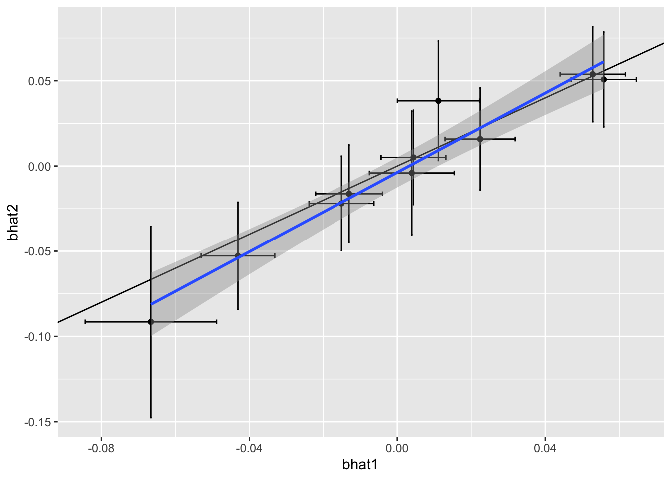
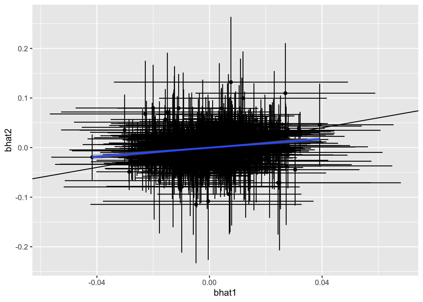
  • The regression of effects across studies might not be 1 even when the true effects are consistent across studies, because power differences can distort the relationship
  • Estimating the observed vs expected replication rates can help to identify if there are systematic differences in effect sizes across studies
  • Estimating the per-variant heterogeneity can estimate if there are any particular variants that have different effect sizes across studies

sessionInfo()
R version 4.3.2 (2023-10-31)
Platform: aarch64-apple-darwin20 (64-bit)
Running under: macOS Ventura 13.6

Matrix products: default
BLAS:   /Library/Frameworks/R.framework/Versions/4.3-arm64/Resources/lib/libRblas.0.dylib 
LAPACK: /Library/Frameworks/R.framework/Versions/4.3-arm64/Resources/lib/libRlapack.dylib;  LAPACK version 3.11.0

locale:
[1] en_GB.UTF-8/en_GB.UTF-8/en_GB.UTF-8/C/en_GB.UTF-8/en_GB.UTF-8

time zone: Europe/London
tzcode source: internal

attached base packages:
[1] stats     graphics  grDevices utils     datasets  methods   base     

other attached packages:
[1] ggplot2_3.4.2 dplyr_1.1.4  

loaded via a namespace (and not attached):
 [1] vctrs_0.6.4       nlme_3.1-163      cli_3.6.1         knitr_1.45       
 [5] rlang_1.1.2       xfun_0.41         generics_0.1.3    jsonlite_1.8.7   
 [9] labeling_0.4.2    glue_1.6.2        colorspace_2.1-0  htmltools_0.5.7  
[13] scales_1.2.1      fansi_1.0.5       rmarkdown_2.25    grid_4.3.2       
[17] munsell_0.5.0     evaluate_0.23     tibble_3.2.1      fastmap_1.1.1    
[21] yaml_2.3.7        lifecycle_1.0.4   compiler_4.3.2    htmlwidgets_1.6.3
[25] pkgconfig_2.0.3   mgcv_1.9-0        farver_2.1.1      lattice_0.21-9   
[29] digest_0.6.33     R6_2.5.1          tidyselect_1.2.0  utf8_1.2.4       
[33] splines_4.3.2     pillar_1.9.0      magrittr_2.0.3    Matrix_1.6-1.1   
[37] withr_2.5.2       tools_4.3.2       gtable_0.3.3