Checking MZ difference model

Background

• Check that mean effects can’t influence MZ dif effects
• That the MZ difference model works for binary traits

Simulate data

• g1 = main effect on y
• g2 = GxE effect with no main effect on y, with an interaction with normally distributed f variable
• g3 = Effect on variance of y
• g4 = Null
• y - continuous variable
• cc - y converted to a binary variable
• cs - cc scaled to have mean 0 and variance 1

library(dplyr)

Attaching package: 'dplyr'

The following objects are masked from 'package:stats':

    filter, lag

The following objects are masked from 'package:base':

    intersect, setdiff, setequal, union

library(ggplot2)
library(tidyr)

n <- 100000
dat <- tibble(
    fid = rep(1:(n/2), each=2), # family id
    id = rep(1:2, n/2),
    g1 = rbinom(n/2, 2, 0.4) %>% rep(., each=2),
    g2 = rbinom(n/2, 2, 0.4) %>% rep(., each=2),
    g3 = rbinom(n/2, 2, 0.4) %>% rep(., each=2),
    g4 = rbinom(n/2, 2, 0.4) %>% rep(., each=2),
    f = rnorm(n),
    v = rnorm(n, 0, g3),
    y = 10 + g1 + f + f * drop(scale(g2)) + v + rnorm(n),
    yr = round(y),
    cc = rbinom(n, 1, plogis(-2 + y)),
    cs = drop(scale(cc))
)
dat

# A tibble: 100,000 × 12
     fid    id    g1    g2    g3    g4      f        v     y    yr    cc     cs
   <int> <int> <int> <int> <int> <int>  <dbl>    <dbl> <dbl> <dbl> <int>  <dbl>
 1     1     1     2     1     1     2  1.55  -0.443   16.4     16     1 0.0515
 2     1     2     2     1     1     2  0.367  0.126   11.2     11     1 0.0515
 3     2     1     0     1     1     0  1.29   0.379   14.3     14     1 0.0515
 4     2     2     0     1     1     0 -0.291  2.96    11.1     11     1 0.0515
 5     3     1     0     1     2     0 -0.891 -0.402    8.49     8     1 0.0515
 6     3     2     0     1     2     0  0.313  0.823   11.3     11     1 0.0515
 7     4     1     0     1     0     0  0.105  0       12.1     12     1 0.0515
 8     4     2     0     1     0     0 -1.72   0        9.25     9     1 0.0515
 9     5     1     0     0     1     2  0.911 -0.405    8.44     8     1 0.0515
10     5     2     0     0     1     2  1.60   0.00454  8.86     9     1 0.0515
# ℹ 99,990 more rows

mean(dat$y)

[1] 10.80035

var(dat$y)

[1] 4.629854

Create MZ data

dat2 <- dat %>% 
    group_by(fid) %>% 
    summarise(
        g1 = g1[1], 
        g2 = g2[1], 
        g3 = g3[1], 
        g4 = g4[1], 
        y2 = (y[1]+y[2])^2,
        y = y[1]-y[2], 
        yrabs = abs(yr[1]-yr[2]), 
        yabs=abs(y), 
        cc=cc[1]-cc[2], 
        cm = mean(cc),
        ccabs=abs(cc),
        cs2=(cs[1]-cs[2])^2,
        cs=cs[1]-cs[2], 
        csabs=abs(cs)
    )
dat2

# A tibble: 50,000 × 15
     fid    g1    g2    g3    g4    y2      y yrabs  yabs    cc    cm ccabs
   <int> <int> <int> <int> <int> <dbl>  <dbl> <dbl> <dbl> <int> <dbl> <int>
 1     1     2     1     1     2  758.  5.22      5 5.22      0     0     0
 2     2     0     1     1     0  645.  3.23      3 3.23      0     0     0
 3     3     0     1     2     0  392. -2.84      3 2.84      0     0     0
 4     4     0     1     0     0  456.  2.84      3 2.84      0     0     0
 5     5     0     0     1     2  299. -0.420     1 0.420     0     0     0
 6     6     0     0     0     0  451. -0.714     1 0.714     0     0     0
 7     7     0     1     1     1  537.  3.64      3 3.64      0     0     0
 8     8     2     1     1     2  493.  4.73      4 4.73      0     0     0
 9     9     0     1     1     1  560. -1.74      2 1.74      0     0     0
10    10     0     0     1     0  414.  2.64      2 2.64      0     0     0
# ℹ 49,990 more rows
# ℹ 3 more variables: cs2 <dbl>, cs <dbl>, csabs <dbl>

This creates the following potential dependent variables for the regression.

• y which is the difference in y between the two MZ twins (as stated in the equation in the paper)
• yabs which is the absolute difference in y between the two MZ twins
• cc which is the difference in cc between the two MZ twins
• ccabs which is the absolute difference in cc between the two MZ twins
• cs which is the difference in the scaled binary variable between the two MZ twins
• cs2 which is the squared difference in the scaled binary variable between the two MZ twins

cm is also generated - the mean of cc for the MZ twins. This is the covariate used in model 2 according to the methods in the paper.

reg <- function(f, dat, what) {
    fo <- as.formula(f)
    o <- lm(fo, data=dat) %>% summary() %>% 
        coef() %>% 
        as.data.frame() %>%
        slice_tail(n=1) %>%
        mutate(what=what, f=f)
    rownames(o) <- NULL
    names(o) <- c("est", "se", "t", "p", "what", "f")
    o %>% select(what, f, est, se, p)
}

o <- bind_rows(
    reg("cc ~ g1", dat, "pop"),
    reg("cc ~ g2", dat, "pop"),
    reg("cc ~ g3", dat, "pop"),
    reg("cc ~ g4", dat, "pop"),
    reg("y ~ g1", dat2, "mz"),
    reg("y ~ g2", dat2, "mz"),
    reg("y ~ g3", dat2, "mz"),
    reg("y ~ g4", dat2, "mz"),
    reg("yabs ~ g1", dat2, "mz"),
    reg("yabs ~ g2", dat2, "mz"),
    reg("yabs ~ g3", dat2, "mz"),
    reg("yabs ~ g4", dat2, "mz"),
    reg("yrabs ~ g1", dat2, "mz"),
    reg("yrabs ~ g2", dat2, "mz"),
    reg("yrabs ~ g3", dat2, "mz"),
    reg("yrabs ~ g4", dat2, "mz"),
    reg("yabs ~ g1 + cm", dat2, "mz"),
    reg("yabs ~ g2 + cm", dat2, "mz"),
    reg("yabs ~ g3 + cm", dat2, "mz"),
    reg("yabs ~ g4 + cm", dat2, "mz"),
    reg("cc ~ g1", dat2, "mz"),
    reg("cc ~ g2", dat2, "mz"),
    reg("cc ~ g3", dat2, "mz"),
    reg("cc ~ g4", dat2, "mz"),
    reg("ccabs ~ g1", dat2, "mz"),
    reg("ccabs ~ g2", dat2, "mz"),
    reg("ccabs ~ g3", dat2, "mz"),
    reg("ccabs ~ g4", dat2, "mz"),
    reg("cs ~ g1", dat2, "mz"),
    reg("cs ~ g2", dat2, "mz"),
    reg("cs ~ g3", dat2, "mz"),
    reg("cs ~ g4", dat2, "mz"),
    reg("csabs ~ g1", dat2, "mz"),
    reg("csabs ~ g2", dat2, "mz"),
    reg("csabs ~ g3", dat2, "mz"),
    reg("csabs ~ g4", dat2, "mz"),
    reg("cs2 ~ g1", dat2, "mz"),
    reg("cs2 ~ g2", dat2, "mz"),
    reg("cs2 ~ g3", dat2, "mz"),
    reg("cs2 ~ g4", dat2, "mz"),
    reg("ccabs ~ g1 + cm", dat2, "mz"),
    reg("ccabs ~ g2 + cm", dat2, "mz"),
    reg("ccabs ~ g3 + cm", dat2, "mz"),
    reg("ccabs ~ g4 + cm", dat2, "mz")
)
o %>% mutate(log10p=-log10(p)) %>% select(what, f, log10p)

   what               f     log10p
1   pop         cc ~ g1 17.2747743
2   pop         cc ~ g2 57.2566871
3   pop         cc ~ g3 10.9891693
4   pop         cc ~ g4  0.3140467
5    mz          y ~ g1  0.3100363
6    mz          y ~ g2  0.8081800
7    mz          y ~ g3  0.2121713
8    mz          y ~ g4  0.7146450
9    mz       yabs ~ g1  0.1442053
10   mz       yabs ~ g2        Inf
11   mz       yabs ~ g3        Inf
12   mz       yabs ~ g4  0.4825420
13   mz      yrabs ~ g1  0.1554996
14   mz      yrabs ~ g2        Inf
15   mz      yrabs ~ g3        Inf
16   mz      yrabs ~ g4  0.8210111
17   mz  yabs ~ g1 + cm  0.5437250
18   mz  yabs ~ g2 + cm  0.5233139
19   mz  yabs ~ g3 + cm  0.4328067
20   mz  yabs ~ g4 + cm  0.5493653
21   mz         cc ~ g1  0.1846266
22   mz         cc ~ g2  0.1032772
23   mz         cc ~ g3  0.4853742
24   mz         cc ~ g4  1.0552000
25   mz      ccabs ~ g1 16.4912008
26   mz      ccabs ~ g2 59.0999919
27   mz      ccabs ~ g3 10.4275082
28   mz      ccabs ~ g4  0.2597902
29   mz         cs ~ g1  0.1846266
30   mz         cs ~ g2  0.1032772
31   mz         cs ~ g3  0.4853742
32   mz         cs ~ g4  1.0552000
33   mz      csabs ~ g1 16.4912008
34   mz      csabs ~ g2 59.0999919
35   mz      csabs ~ g3 10.4275082
36   mz      csabs ~ g4  0.2597902
37   mz        cs2 ~ g1 16.4912008
38   mz        cs2 ~ g2 59.0999919
39   mz        cs2 ~ g3 10.4275082
40   mz        cs2 ~ g4  0.2597902
41   mz ccabs ~ g1 + cm 36.8960428
42   mz ccabs ~ g2 + cm 37.0215620
43   mz ccabs ~ g3 + cm 36.8091556
44   mz ccabs ~ g4 + cm 36.9677338

Observations

• The MZ difference model does not work for the difference of y
• The MZ difference model works for continuous traits as expected when using the absolute difference in the trait (yabs). i.e.
  • The main effect does not associate with MZ dif
  • The GxE effect does associate with MZ dif
  • The variance effect does associate with MZ dif
• The MZ difference model does not work for the difference of the binary trait cc
• Using the absolute difference in the binary trait (ccabs)
  • Picks up the GxE effect and the variance effect
  • But it also picks up the main effect which it is not supposed to do

reg2 <- function(f, dat, what) {
    fo <- as.formula(f)
    o <- glm(fo, data=dat, family="binomial") %>% summary() %>% 
        coef() %>% 
        as.data.frame() %>%
        slice_tail(n=1) %>%
        mutate(what=what, f=f)
    rownames(o) <- NULL
    names(o) <- c("est", "se", "t", "p", "what", "f")
    o %>% select(what, f, est, se, p)
}
o <- bind_rows(
    reg2("ccabs ~ g1", dat2, "mz"),
    reg2("ccabs ~ g2", dat2, "mz"),
    reg2("ccabs ~ g3", dat2, "mz"),
    reg2("ccabs ~ g4", dat2, "mz"),
    reg2("ccabs ~ g1 + cm", dat2, "mz"),
    reg2("ccabs ~ g2 + cm", dat2, "mz"),
    reg2("ccabs ~ g3 + cm", dat2, "mz"),
    reg2("ccabs ~ g4 + cm", dat2, "mz")
)
o %>% select(what, f, p) %>% mutate(p=-log10(p))

  what               f          p
1   mz      ccabs ~ g1 15.5448674
2   mz      ccabs ~ g2 49.1431818
3   mz      ccabs ~ g3 10.1598219
4   mz      ccabs ~ g4  0.2597595
5   mz ccabs ~ g1 + cm 25.0419829
6   mz ccabs ~ g2 + cm 16.5004672
7   mz ccabs ~ g3 + cm 26.2644940
8   mz ccabs ~ g4 + cm 29.5233782

summary(lm(y ~ f * g2, dat))

Call:
lm(formula = y ~ f * g2, data = dat)

Residuals:
    Min      1Q  Median      3Q     Max 
-8.5041 -1.0189 -0.0054  1.0200  9.9971 

Coefficients:
             Estimate Std. Error  t value Pr(>|t|)    
(Intercept) 10.792120   0.007755 1391.600   <2e-16 ***
f           -0.153508   0.007702  -19.930   <2e-16 ***
g2           0.006775   0.007323    0.925    0.355    
f:g2         1.445652   0.007259  199.158   <2e-16 ***
---
Signif. codes:  0 '***' 0.001 '**' 0.01 '*' 0.05 '.' 0.1 ' ' 1

Residual standard error: 1.609 on 99996 degrees of freedom
Multiple R-squared:  0.4406,    Adjusted R-squared:  0.4405 
F-statistic: 2.625e+04 on 3 and 99996 DF,  p-value: < 2.2e-16

tapply(dat$y, dat$g2, var)

        0         1         2 
 2.634606  4.248730 10.238937 

tapply(dat$y, dat$g3, var)

       0        1        2 
3.485533 4.539930 7.455329 

tapply(dat2$yabs, dat2$g2, mean)

       0        1        2 
1.575893 2.168476 3.507917 

tapply(dat2$yabs, dat2$g3, mean)

       0        1        2 
1.810245 2.189781 2.914333 

Trait skewness

n <- 100000
dat <- tibble(
    fid = rep(1:(n/2), each=2), # family id
    id = rep(1:2, n/2),
    g1 = rbinom(n/2, 2, 0.4) %>% rep(., each=2),
    g2 = rbinom(n/2, 2, 0.4) %>% rep(., each=2),
    g3 = rbinom(n/2, 2, 0.4) %>% rep(., each=2),
    g4 = rbinom(n/2, 2, 0.4) %>% rep(., each=2),
    f = rnorm(n),
    v = rnorm(n, 0, g3),
    y = (10 + g1 + f + f * drop(scale(g2)) + v + rnorm(n))^1.2,
    yr = round(y),
    cc = rbinom(n, 1, plogis(-2 + y)),
    cs = drop(scale(cc))
)

Warning in rbinom(n, 1, plogis(-2 + y)): NAs produced

dat

# A tibble: 100,000 × 12
     fid    id    g1    g2    g3    g4       f      v     y    yr    cc     cs
   <int> <int> <int> <int> <int> <int>   <dbl>  <dbl> <dbl> <dbl> <int>  <dbl>
 1     1     1     1     1     0     1  0.363   0      19.8    20     1 0.0247
 2     1     2     1     1     0     1  1.50    0      19.8    20     1 0.0247
 3     2     1     1     0     1     2 -1.75   -2.99   11.7    12     1 0.0247
 4     2     2     1     0     1     2 -0.373  -2.33   14.7    15     1 0.0247
 5     3     1     1     1     2     0 -0.782  -0.945  14.2    14     1 0.0247
 6     3     2     1     1     2     0  0.786   0.380  18.4    18     1 0.0247
 7     4     1     2     0     1     0  0.925  -0.726  21.2    21     1 0.0247
 8     4     2     2     0     1     0 -0.0610 -0.495  20.1    20     1 0.0247
 9     5     1     1     1     1     0  1.18    0.582  18.3    18     1 0.0247
10     5     2     1     1     1     0 -0.268   0.853  21.0    21     1 0.0247
# ℹ 99,990 more rows

Create MZ data

dat2 <- dat %>% 
    group_by(fid) %>% 
    summarise(
        g1 = g1[1], 
        g2 = g2[1], 
        g3 = g3[1], 
        g4 = g4[1], 
        y2 = (y[1]+y[2])^2,
        ym = mean(c(y[1], y[2])),
        y = y[1]-y[2], 
        yrabs = abs(yr[1]-yr[2]), 
        yabs=abs(y), 
        cc=cc[1]-cc[2], 
        cm = mean(cc),
        ccabs=abs(cc),
        cs2=(cs[1]-cs[2])^2,
        cs=cs[1]-cs[2], 
        csabs=abs(cs)
    )
dat2

# A tibble: 50,000 × 16
     fid    g1    g2    g3    g4    y2    ym       y yrabs   yabs    cc    cm
   <int> <int> <int> <int> <int> <dbl> <dbl>   <dbl> <dbl>  <dbl> <int> <dbl>
 1     1     1     1     0     1 1569.  19.8  0.0214     0 0.0214     0     0
 2     2     1     0     1     2  699.  13.2 -2.93       3 2.93       0     0
 3     3     1     1     2     0 1062.  16.3 -4.13       4 4.13       0     0
 4     4     2     0     1     0 1706.  20.7  1.06       1 1.06       0     0
 5     5     1     1     1     0 1539.  19.6 -2.71       3 2.71       0     0
 6     6     0     2     1     1 1407.  18.8  4.94       5 4.94       0     0
 7     7     1     0     0     1 1190.  17.3 -2.01       2 2.01       0     0
 8     8     1     0     0     1 1251.  17.7 -1.55       1 1.55       0     0
 9     9     0     0     1     1 1078.  16.4 -0.602      1 0.602      0     0
10    10     2     2     1     1 2939.  27.1  1.17       1 1.17       0     0
# ℹ 49,990 more rows
# ℹ 4 more variables: ccabs <int>, cs2 <dbl>, cs <dbl>, csabs <dbl>

o <- bind_rows(
    reg("y ~ g1", dat, "pop"),
    reg("y ~ g2", dat, "pop"),
    reg("y ~ g3", dat, "pop"),
    reg("y ~ g4", dat, "pop"),
    reg("y ~ g1", dat2, "mz"),
    reg("y ~ g2", dat2, "mz"),
    reg("y ~ g3", dat2, "mz"),
    reg("y ~ g4", dat2, "mz"),
    reg("yabs ~ g1", dat2, "mz"),
    reg("yabs ~ g2", dat2, "mz"),
    reg("yabs ~ g3", dat2, "mz"),
    reg("yabs ~ g4", dat2, "mz"),
    reg("yrabs ~ g1", dat2, "mz"),
    reg("yrabs ~ g2", dat2, "mz"),
    reg("yrabs ~ g3", dat2, "mz"),
    reg("yrabs ~ g4", dat2, "mz"),
    reg("yabs ~ g1 + cm", dat2, "mz"),
    reg("yabs ~ g2 + cm", dat2, "mz"),
    reg("yabs ~ g3 + cm", dat2, "mz"),
    reg("yabs ~ g4 + cm", dat2, "mz")
)
o %>% mutate(log10p=-log10(p)) %>% select(what, f, log10p)

   what              f     log10p
1   pop         y ~ g1        Inf
2   pop         y ~ g2 2.44671037
3   pop         y ~ g3 3.90724985
4   pop         y ~ g4 0.29606699
5    mz         y ~ g1 0.08322533
6    mz         y ~ g2 0.13162987
7    mz         y ~ g3 0.07244880
8    mz         y ~ g4 0.19959080
9    mz      yabs ~ g1 2.82370784
10   mz      yabs ~ g2        Inf
11   mz      yabs ~ g3        Inf
12   mz      yabs ~ g4 0.08054570
13   mz     yrabs ~ g1 2.80228703
14   mz     yrabs ~ g2        Inf
15   mz     yrabs ~ g3        Inf
16   mz     yrabs ~ g4 0.10686095
17   mz yabs ~ g1 + cm 3.75871309
18   mz yabs ~ g2 + cm 3.38758782
19   mz yabs ~ g3 + cm 4.31651544
20   mz yabs ~ g4 + cm 3.75068702

cor(dat2$ym, dat2$y, use="pair")

[1] 0.0005741118

Make a Poisson model and then normalise

inormal <- function(x) {
    x <- x + rnorm(length(x), 0, 1e-10)
    qnorm((rank(x, na.last = "keep") - 0.5) / sum(!is.na(x)))
}

n <- 100000
dat <- tibble(
    fid = rep(1:(n/2), each=2), # family id
    id = rep(1:2, n/2),
    g1 = rbinom(n/2, 2, 0.4) %>% rep(., each=2),
    g2 = rbinom(n/2, 2, 0.4) %>% rep(., each=2),
    g3 = rbinom(n/2, 2, 0.4) %>% rep(., each=2),
    g4 = rbinom(n/2, 2, 0.4) %>% rep(., each=2),
    f = rnorm(n),
    e = rnorm(n),
    v = rnorm(n, 0, g3 * 0.1),
    y = drop(scale(g1) * 0.1 + f * 0.1 + f * drop(scale(g2)) * 0.1 + v + e),
    l = drop(exp(scale(y) * 0.1)),
    score = rpois(n, l),
    score_norm = inormal(score),
    l_norm = inormal(l)
)
dat

# A tibble: 100,000 × 14
     fid    id    g1    g2    g3    g4       f      e       v       y     l
   <int> <int> <int> <int> <int> <int>   <dbl>  <dbl>   <dbl>   <dbl> <dbl>
 1     1     1     2     1     1     0  0.476  -0.155 -0.0560  0.0236 1.00 
 2     1     2     2     1     1     0 -0.545   0.591 -0.253   0.441  1.04 
 3     2     1     0     1     2     1 -0.539   1.14   0.213   1.17   1.12 
 4     2     2     0     1     2     1 -1.79    0.810  0.0542  0.517  1.05 
 5     3     1     1     1     0     1 -0.0322  0.926  0       0.951  1.10 
 6     3     2     1     1     0     1 -0.634  -1.39   0      -1.44   0.868
 7     4     1     1     0     1     2 -0.916   1.43  -0.0631  1.41   1.15 
 8     4     2     1     0     1     2  0.620   0.690  0.127   0.837  1.08 
 9     5     1     0     1     1     2  0.131  -0.337  0.0989 -0.336  0.967
10     5     2     0     1     1     2 -0.113   0.874 -0.0615  0.682  1.07 
# ℹ 99,990 more rows
# ℹ 3 more variables: score <int>, score_norm <dbl>, l_norm <dbl>

hist(dat$score)

hist(dat$score_norm)

cor(dat$score, dat$score_norm, use="pair")

[1] 0.9121883

cor(dat$score, dat$l)

[1] 0.09660049

cor(dat$y, dat$l)

[1] 0.9975233

mean(dat$y)

[1] 0.006094577

var(dat$l)

[1] 0.01015692

mean(dat$l)

[1] 1.005014

Create MZ data

dat2 <- dat %>% 
    group_by(fid) %>% 
    summarise(
        g1 = g1[1], 
        g2 = g2[1], 
        g3 = g3[1], 
        g4 = g4[1], 
        y2 = (y[1]+y[2])^2,
        y = y[1]-y[2], 
        l = abs(l[1]-l[2]), 
        l_norm = abs(l_norm[1]-l_norm[2]),
        yabs = abs(y), 
        score = abs(score[1]-score[2]), 
        ms = mean(score_norm),
        score_norm = abs(score_norm[1]-score_norm[2])
    )
dat2

# A tibble: 50,000 × 13
     fid    g1    g2    g3    g4      y2      y      l l_norm  yabs score
   <int> <int> <int> <int> <int>   <dbl>  <dbl>  <dbl>  <dbl> <dbl> <int>
 1     1     2     1     1     0  0.216  -0.417 0.0419  0.409 0.417     2
 2     2     0     1     2     1  2.84    0.652 0.0695  0.628 0.652     1
 3     3     1     1     0     1  0.239   2.39  0.230   2.34  2.39      0
 4     4     1     0     1     2  5.03    0.569 0.0624  0.561 0.569     2
 5     5     0     1     1     2  0.120  -1.02  0.102   0.998 1.02      1
 6     6     0     1     1     0  0.229   1.28  0.129   1.25  1.28      2
 7     7     1     1     1     1  0.297  -0.260 0.0262  0.257 0.260     1
 8     8     1     1     1     1  1.19   -0.660 0.0683  0.640 0.660     2
 9     9     0     1     1     0  0.0839 -0.709 0.0705  0.697 0.709     1
10    10     0     0     0     0 11.3     2.45  0.204   2.42  2.45      1
# ℹ 49,990 more rows
# ℹ 2 more variables: ms <dbl>, score_norm <dbl>

hist(dat2$l)

hist(dat2$y, breaks=100)

hist(dat2$score)

hist(dat2$ms)

hist(dat2$score_norm, breaks=100)

o <- bind_rows(
    reg("y ~ g1", dat, "pop"),
    reg("y ~ g2", dat, "pop"),
    reg("y ~ g3", dat, "pop"),
    reg("y ~ g4", dat, "pop"),
    reg("y ~ g1", dat2, "mz"),
    reg("y ~ g2", dat2, "mz"),
    reg("y ~ g3", dat2, "mz"),
    reg("y ~ g4", dat2, "mz"),
    reg("yabs ~ g1", dat2, "mz"),
    reg("yabs ~ g2", dat2, "mz"),
    reg("yabs ~ g3", dat2, "mz"),
    reg("yabs ~ g4", dat2, "mz"),
    reg("l ~ g1", dat2, "mz"),
    reg("l ~ g2", dat2, "mz"),
    reg("l ~ g3", dat2, "mz"),
    reg("l ~ g4", dat2, "mz"),
    reg("l_norm ~ g1", dat2, "mz"),
    reg("l_norm ~ g2", dat2, "mz"),
    reg("l_norm ~ g3", dat2, "mz"),
    reg("l_norm ~ g4", dat2, "mz"),
    reg("score ~ g1", dat2, "mz"),
    reg("score ~ g2", dat2, "mz"),
    reg("score ~ g3", dat2, "mz"),
    reg("score ~ g4", dat2, "mz"),
    reg("score_norm ~ g1", dat2, "mz"),
    reg("score_norm ~ g2", dat2, "mz"),
    reg("score_norm ~ g3", dat2, "mz"),
    reg("score_norm ~ g4", dat2, "mz")
)
o %>% mutate(log10p=-log10(p)) %>% select(what, f, log10p)

   what               f       log10p
1   pop          y ~ g1 223.49845803
2   pop          y ~ g2   0.34714511
3   pop          y ~ g3   0.25819938
4   pop          y ~ g4   0.64395220
5    mz          y ~ g1   0.03632132
6    mz          y ~ g2   0.38132042
7    mz          y ~ g3   1.00079267
8    mz          y ~ g4   0.68887829
9    mz       yabs ~ g1   0.34922634
10   mz       yabs ~ g2   1.53015386
11   mz       yabs ~ g3   0.92366698
12   mz       yabs ~ g4   0.27304613
13   mz          l ~ g1   3.60869823
14   mz          l ~ g2   1.67822720
15   mz          l ~ g3   0.90363896
16   mz          l ~ g4   0.33315183
17   mz     l_norm ~ g1   0.30614450
18   mz     l_norm ~ g2   1.54241162
19   mz     l_norm ~ g3   0.93572455
20   mz     l_norm ~ g4   0.26916190
21   mz      score ~ g1   0.01469387
22   mz      score ~ g2   0.45762861
23   mz      score ~ g3   0.74625997
24   mz      score ~ g4   0.02614553
25   mz score_norm ~ g1   0.19612508
26   mz score_norm ~ g2   0.75161526
27   mz score_norm ~ g3   0.47842950
28   mz score_norm ~ g4   0.30320457

Run simulations with more replications

The general model

• y is a continuous variable which relates to the underlying normal liability
• ysq is the square of y, to introduce skewness
• ysq_norm is the inverse rank transformed ysq to try to rescue the skewness
• l is the exponentiated liability which will eventually give rise to the Poisson distributed variable
• l_norm is the inverse rank transformed l to try to rescue the skewness
• score is the Poisson distributed variable arising from the underlying normal liability. This aims to represent the depression / anxiety distributions
• score_norm is the inverse rank transformed score to try to rescue the skewness. Note that small amounts of noise are introduced to avoid ties

dgm <- function(n, b1, b2, b3, b4, bf, bf2) {
    dat <- tibble(
        fid = rep(1:(n/2), each=2), # family id
        id = rep(1:2, n/2),
        g1 = rbinom(n/2, 2, 0.4) %>% rep(., each=2),
        g2 = rbinom(n/2, 2, 0.4) %>% rep(., each=2),
        g3 = rbinom(n/2, 2, 0.4) %>% rep(., each=2),
        g4 = rbinom(n/2, 2, 0.4) %>% rep(., each=2),
        f = rnorm(n),
        e = rnorm(n),
        v = rnorm(n, 0, g3 * b3),
        covar = rnorm(n, 0, 0.5),
        y = drop(covar + scale(g1) * b1 + scale(g2) * b2 + f * bf + f * drop(scale(g2)) * bf2 + v + e + scale(g4) * b4),
        ysq = y^2,
        ysq_norm = inormal(ysq),
        l = drop(exp(scale(y) * 0.1)),
        l_norm = inormal(l),
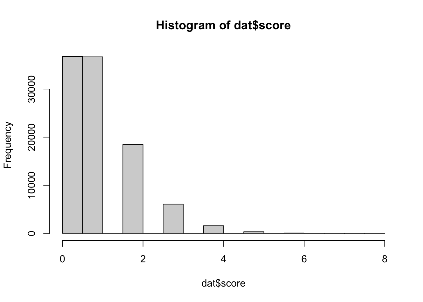
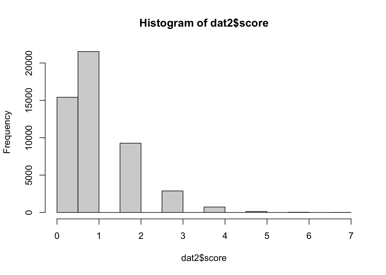
        score = rpois(n, l),
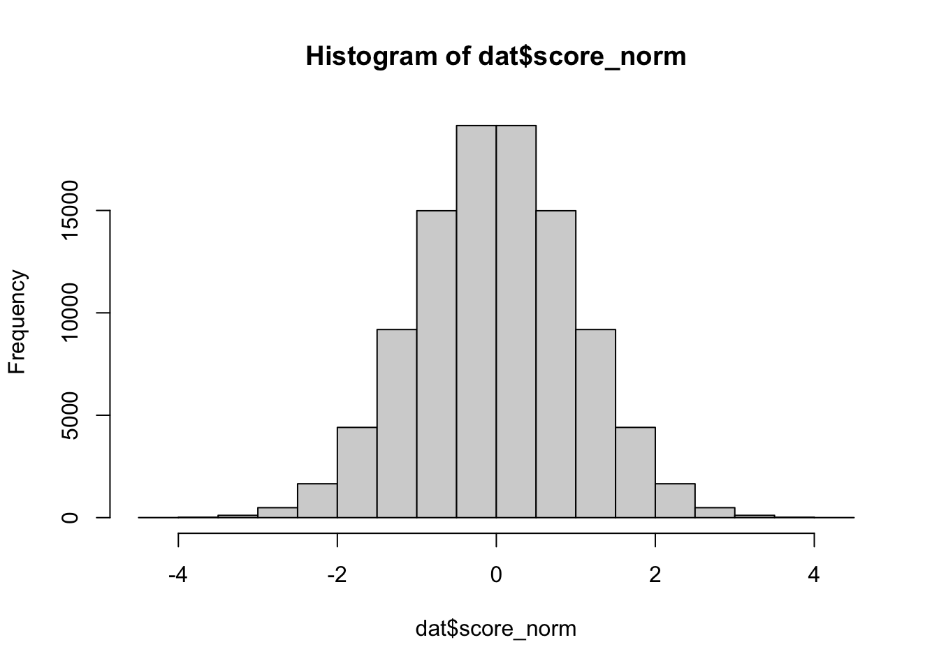
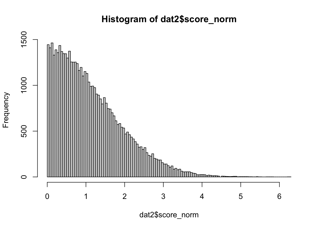
        score_norm = inormal(score),
        score_res = residuals(lm(y ~ covar)),
        score_res_norm = inormal(score_res)
    )

    dat2 <- dat %>% 
        group_by(fid) %>% 
        summarise(
            g1 = g1[1], 
            g2 = g2[1], 
            g3 = g3[1], 
            g4 = g4[1], 
            yraw = y[1]-y[2], 
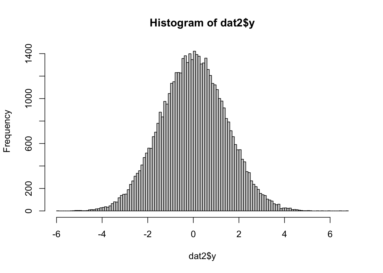
            y = abs(yraw), 
            ysq = abs(ysq[1]+ysq[2]),
            ysq_norm = abs(ysq_norm[1]+ysq_norm[2]),
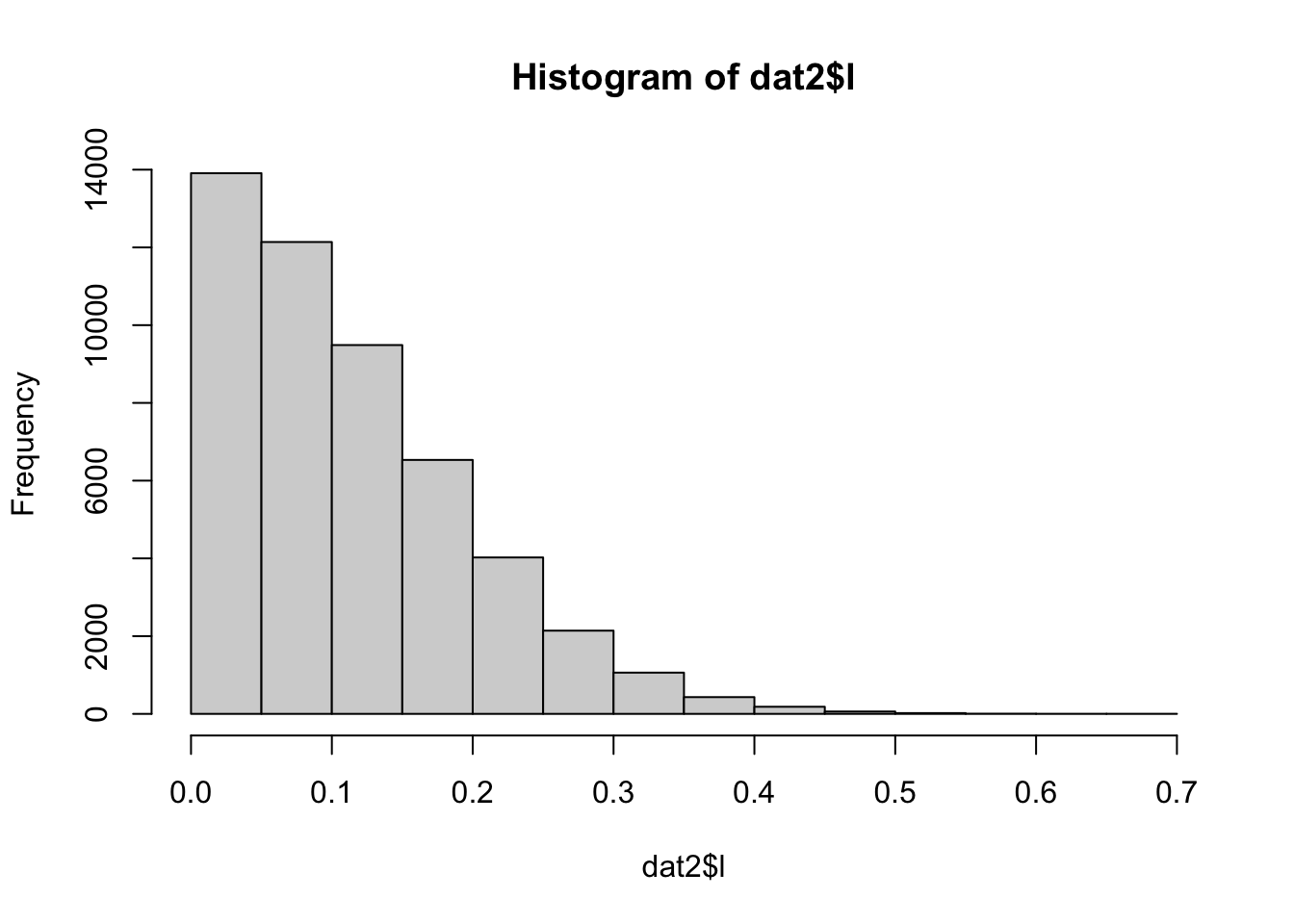
            l = abs(l[1]-l[2]), 
            l_norm = abs(l_norm[1]-l_norm[2]),
            score = abs(score[1]-score[2]), 
            score_norm = abs(score_norm[1]-score_norm[2]),
            score_res = abs(score_res[1]-score_res[2]),
            score_res_norm = abs(score_res_norm[1]-score_res_norm[2])
        )
    return(list(dat=dat, dat2=dat2))
}

est <- function(out) {
    dat <- out$dat
    dat2 <- out$dat2
    o <- bind_rows(
        reg("y ~ g1", dat, "pop"),
        reg("y ~ g2", dat, "pop"),
        reg("y ~ g3", dat, "pop"),
        reg("y ~ g4", dat, "pop"),
        reg("yraw ~ g1", dat2, "mz"),
        reg("yraw ~ g2", dat2, "mz"),
        reg("yraw ~ g3", dat2, "mz"),
        reg("yraw ~ g4", dat2, "mz"),
        reg("y ~ g1", dat2, "mz"),
        reg("y ~ g2", dat2, "mz"),
        reg("y ~ g3", dat2, "mz"),
        reg("y ~ g4", dat2, "mz"),
        reg("ysq ~ g1", dat2, "mz"),
        reg("ysq ~ g2", dat2, "mz"),
        reg("ysq ~ g3", dat2, "mz"),
        reg("ysq ~ g4", dat2, "mz"),
        reg("ysq_norm ~ g1", dat2, "mz"),
        reg("ysq_norm ~ g2", dat2, "mz"),
        reg("ysq_norm ~ g3", dat2, "mz"),
        reg("ysq_norm ~ g4", dat2, "mz"),
        reg("l ~ g1", dat2, "mz"),
        reg("l ~ g2", dat2, "mz"),
        reg("l ~ g3", dat2, "mz"),
        reg("l ~ g4", dat2, "mz"),
        reg("l_norm ~ g1", dat2, "mz"),
        reg("l_norm ~ g2", dat2, "mz"),
        reg("l_norm ~ g3", dat2, "mz"),
        reg("l_norm ~ g4", dat2, "mz"),
        reg("score ~ g1", dat2, "mz"),
        reg("score ~ g2", dat2, "mz"),
        reg("score ~ g3", dat2, "mz"),
        reg("score ~ g4", dat2, "mz"),
        reg("score_norm ~ g1", dat2, "mz"),
        reg("score_norm ~ g2", dat2, "mz"),
        reg("score_norm ~ g3", dat2, "mz"),
        reg("score_norm ~ g4", dat2, "mz"),
        reg("score_res ~ g1", dat2, "mz"),
        reg("score_res ~ g2", dat2, "mz"),
        reg("score_res ~ g3", dat2, "mz"),
        reg("score_res ~ g4", dat2, "mz"),
        reg("score_res_norm ~ g1", dat2, "mz"),
        reg("score_res_norm ~ g2", dat2, "mz"),
        reg("score_res_norm ~ g3", dat2, "mz"),
        reg("score_res_norm ~ g4", dat2, "mz")
    )
    return(o)
}

Run the sims

res <- lapply(1:100, \(i) {
    out <- dgm(10000, 0.3, 0, 0.3, 0, 0.3, 0.3)
    est(out) %>% mutate(i=i)
}) %>% bind_rows()

Re-label

res <- res %>% separate(f, c("trait", "g"), sep=" ~ ", remove=FALSE)
res$g[res$g == "g1"] <- "Main"
res$g[res$g == "g2"] <- "GxE"
res$g[res$g == "g3"] <- "Var"
res$g[res$g == "g4"] <- "Null"

res$trait[res$trait == "yraw"] <- "yraw"
res$trait[res$trait == "y"] <- "Normal liability"
res$trait[res$trait == "ysq"] <- "Normal liability squared"
res$trait[res$trait == "ysq_norm"] <- "Normal liability squared (INT)"
res$trait[res$trait == "l"] <- "Exponentiated liability"
res$trait[res$trait == "l_norm"] <- "Exponentiated liability (INT)"
res$trait[res$trait == "score"] <- "Poisson of liability"
res$trait[res$trait == "score_norm"] <- "Poisson of liability (INT)"
res$trait[res$trait == "score_res"] <- "Residuals of Poisson"
res$trait[res$trait == "score_res_norm"] <- "Residuals of Poisson (INT)"

Evaluate performance of variance estimates on power and bias. Expect that Main and Null should be null in the MZ difference model, and GxE and Var should be non-null.

ggplot(res %>% filter(what =="mz" & trait != "yraw") %>% group_by(trait) %>% mutate(est = est/max(est)), aes(x=g, y=est)) + 
    geom_boxplot(aes(fill=g)) +
    theme(axis.text.x = element_text(angle = 90, hjust = 1, vjust = 0.5), legend.position="none") +
    scale_fill_brewer(palette="Set3") +
    geom_hline(yintercept=0, linetype="dashed") +
    facet_grid(. ~ trait, scale="free_y", labeller = label_wrap_gen()) +
    labs(y = "Relative effect size", x="", fill="")

ggsave(file="mz_diff.pdf", width=12, height=8)

ggplot(res %>% filter(what =="mz" & trait != "yraw"), aes(x=trait, y=-log10(p))) + 
    geom_boxplot(aes(fill=g)) +
    theme(axis.text.x = element_text(angle = 90, hjust = 1, vjust = 0.5)) +
    scale_fill_brewer(palette="Set3")

res %>% group_by(what, f, g, trait) %>% summarise(power = sum(p < 0.05)) %>%
    ungroup %>%
    {
    ggplot(., aes(x=g, y=power)) + 
        geom_bar(stat="identity", aes(fill=g), position="dodge") +
        theme(axis.text.x = element_text(angle = 90, hjust = 1, vjust = 0.5)) +
        scale_fill_brewer(palette="Set3") +
        facet_grid(. ~ trait)
    }

`summarise()` has grouped output by 'what', 'f', 'g'. You can override using
the `.groups` argument.

Summary

• Inverse rank transformation of most traits rescues the MZ difference model
• Inverse rank transformation of the Poisson variable does not seem to work - it erases the variance effects and there is some bias remaining for the main effect

---

sessionInfo()

R version 4.3.3 (2024-02-29)
Platform: aarch64-apple-darwin20 (64-bit)
Running under: macOS Ventura 13.6

Matrix products: default
BLAS:   /Library/Frameworks/R.framework/Versions/4.3-arm64/Resources/lib/libRblas.0.dylib 
LAPACK: /Library/Frameworks/R.framework/Versions/4.3-arm64/Resources/lib/libRlapack.dylib;  LAPACK version 3.11.0

locale:
[1] en_GB.UTF-8/en_GB.UTF-8/en_GB.UTF-8/C/en_GB.UTF-8/en_GB.UTF-8

time zone: Europe/London
tzcode source: internal

attached base packages:
[1] stats     graphics  grDevices utils     datasets  methods   base     

other attached packages:
[1] tidyr_1.3.0   ggplot2_3.4.2 dplyr_1.1.4  

loaded via a namespace (and not attached):
 [1] vctrs_0.6.5        cli_3.6.2          knitr_1.45         rlang_1.1.3       
 [5] xfun_0.42          purrr_1.0.2        generics_0.1.3     textshaping_0.3.7 
 [9] jsonlite_1.8.8     labeling_0.4.2     glue_1.7.0         colorspace_2.1-0  
[13] htmltools_0.5.7    ragg_1.2.6         scales_1.2.1       fansi_1.0.6       
[17] rmarkdown_2.26     grid_4.3.3         munsell_0.5.0      evaluate_0.23     
[21] tibble_3.2.1       fastmap_1.1.1      yaml_2.3.8         lifecycle_1.0.4   
[25] compiler_4.3.3     RColorBrewer_1.1-3 htmlwidgets_1.6.3  pkgconfig_2.0.3   
[29] systemfonts_1.0.5  farver_2.1.1       digest_0.6.34      R6_2.5.1          
[33] tidyselect_1.2.0   utf8_1.2.4         pillar_1.9.0       magrittr_2.0.3    
[37] withr_3.0.0        tools_4.3.3        gtable_0.3.3