Differences in cancer prevalence and heritability

Background

Richard Peto points out, and later George Davey Smith, that cancer prevalence is very different across geographical regions and across time periods within geographical regions. Such systematic differences are too rapid to be explained by genetic factors, and too structured to be explained by chance. When comparing the rates of cancer between the highest 20% and lowest 20% prevalence, they suggest that ~80% of cancer is due to modifiable risk factors. Similar rates for mortality differences, meaning that it’s plausible that this isn’t due to differential rates of cancer detection.

How does this square with heritability? It implies that 80% of the variance in cancer is due to a set of modifiable factors. But if h2 is higher than 20% then is this possible?

Consider smoking and lung cancer. If smoking is partially genetic and partially environmental, what happens in this high vs low prevalence calculation?

library(dplyr)

Attaching package: 'dplyr'

The following objects are masked from 'package:stats':

    filter, lag

The following objects are masked from 'package:base':

    intersect, setdiff, setequal, union

library(tidyr)
library(ggplot2)

Positive control, lets make it so that 80% of the trait is due to environment and 20% random chance

n <- 10000

dat <- bind_rows(
    tibble(
        envir = rbinom(n, 1, 0) * 10,
        cancer = rbinom(n, 1, plogis(-1.9 + envir)),
        cat="low"
    ),
    tibble(
        envir = rbinom(n, 1, 0.8) * 10,
        cancer = rbinom(n, 1, plogis(-1.9 + envir)),
        cat="high"
    )
) 

cor(dat$envir[dat$cat=="high"], dat$cancer[dat$cat=="high"])^2

[1] 0.8200225

cor(dat$envir, dat$cancer)^2

[1] 0.7139614

dat %>%
    group_by(cat) %>%
    summarise(prev_cancer = sum(cancer) / n(), mean_env = mean(envir))

# A tibble: 2 × 3
  cat   prev_cancer mean_env
  <chr>       <dbl>    <dbl>
1 high        0.824     7.94
2 low         0.135     0   

Now introduce genetic variance

There is a heritability of 50% which is independent of environmental effect

dat <- bind_rows(
    tibble(
        envir = rbinom(n, 1, 0) * 10,
        g = rnorm(n),
        cancer = rbinom(n, 1, plogis(-1.9 + envir + g*10)),
        cat="low"
    ),
    tibble(
        envir = rbinom(n, 1, 0.8) * 10,
        g = rnorm(n),
        cancer = rbinom(n, 1, plogis(-1.9 + envir + g*10)),
        cat="high"
    )
) 
cor(dat$g[dat$cat=="high"], dat$cancer[dat$cat=="high"])^2

[1] 0.4576331

dat %>%
    group_by(cat) %>%
    summarise(prev_cancer = sum(cancer) / n(), mean_env = mean(envir))

# A tibble: 2 × 3
  cat   prev_cancer mean_env
  <chr>       <dbl>    <dbl>
1 high        0.714     8.03
2 low         0.436     0   

That raises the prevalence in the low group. Now lets make the genetic factor mediated through behaviour

dat <- bind_rows(
    tibble(
        g = rnorm(n),
        e = rnorm(n, sd=1),
        envir = rbinom(n, 1, plogis(g + e)) * 10,
        cancer = rbinom(n, 1, plogis(-1.9 + envir)),
        cat="low"
    ),
    tibble(
        g = rnorm(n),
        e = rnorm(n, sd=10),
        envir = rbinom(n, 1, plogis(g + e)) * 10,
        cancer = rbinom(n, 1, plogis(-1.9 + envir)),
        cat="high"
    )
) 
cor(dat$g[dat$cat=="high"], dat$cancer[dat$cat=="high"])^2

[1] 0.002550874

dat %>%
    group_by(cat) %>%
    summarise(prev_cancer = sum(cancer) / n(), mean_env = mean(envir))

# A tibble: 2 × 3
  cat   prev_cancer mean_env
  <chr>       <dbl>    <dbl>
1 high        0.571     5.04
2 low         0.566     4.94

I think you need a G x E interaction. You might have a high liability to smoke but the availability of cigarettes is very low, so that genetic variance cannot manifest. How does that appear as a statistical model? It will be the genetic risk on outcome + environmental risk on outcome, multiplied by accessibility to the outcome

dat <- bind_rows(
    tibble(
        g = rbeta(n, 3, 1),
        accessibility = rbinom(n, 1, 0.001),
        envir = rbinom(n, 1, g * accessibility),
        cancer = rbinom(n, 1, plogis(-1.9 + envir * 10)),
        cat="low"
    ),
    tibble(
        g = rbeta(n, 3, 1),
        accessibility = rbinom(n, 1, 0.999),
        envir = rbinom(n, 1, g * accessibility),
        cancer = rbinom(n, 1, plogis(-1.9 + envir * 10)),
        cat="high"
    )
) 
cor(dat$g[dat$cat=="high"], dat$cancer[dat$cat=="high"])^2

[1] 0.1662182

cor(dat$g[dat$cat=="low"], dat$cancer[dat$cat=="low"])^2

[1] 2.929504e-05

dat %>%
    group_by(cat) %>%
    summarise(prev_cancer = sum(cancer) / n(), mean_env = mean(envir), mean_acc=mean(accessibility), mean_env_p = mean(plogis(envir)))

# A tibble: 2 × 5
  cat   prev_cancer mean_env mean_acc mean_env_p
  <chr>       <dbl>    <dbl>    <dbl>      <dbl>
1 high        0.779   0.749    0.999       0.673
2 low         0.132   0.0003   0.0005      0.500

But here the heritability is limited to the non-genetic variance.

Allow liability variance to change

• Simulate twins
• Estimate heritability in high and low prevalence groups
• Estimate fraction of cases change

15-30x more likely to get lung cancer if you smoke 1.5% of non-smokers get lung cancer 12% of smokers get lung cancer

n <- 1000000
dat <- bind_rows(
    tibble(
        g = rnorm(n, sd=1),
        e = rnorm(n, sd=1),
        smoking = 2,
        liability = -4 + g + e + smoking,
        cancer = rbinom(n, 1, plogis(liability)),
        cat="high"
    ),
    tibble(
        g = rnorm(n, sd=1),
        e = rnorm(n, sd=1),
        smoking = 0,
        liability = -4 + g + e + smoking,
        cancer = rbinom(n, 1, plogis(liability)),
        cat="low"
    ),
)

group_by(dat, cat) %>%
    summarise(
        prev_cancer = sum(cancer) / n(),
        mean_g = mean(g),
        mean_e = mean(e),
        mean_smoking = mean(smoking),
        mean_liability = mean(liability),
        h2 = cor(g, liability)^2,
        h2obs = cor(g, cancer)^2,
    )

# A tibble: 2 × 8
  cat   prev_cancer    mean_g    mean_e mean_smoking mean_liability    h2  h2obs
  <chr>       <dbl>     <dbl>     <dbl>        <dbl>          <dbl> <dbl>  <dbl>
1 high       0.184  -0.00131  -0.000625            2          -2.00 0.499 0.0904
2 low        0.0405  0.000666 -0.000439            0          -4.00 0.499 0.0311

cor(dat$cancer, dat$g)^2

[1] 0.05730214

cor(dat$smoking, dat$cancer)^2

[1] 0.05152482

ggplot(dat, aes(x=liability)) +
geom_density(aes(fill=cat), alpha=0.5)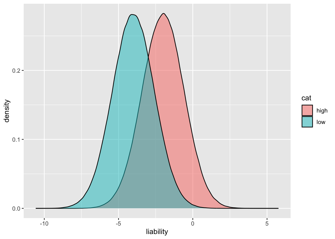

Twin model

make_families <- function(af, nfam, beta) {
    nsnp <- length(af)
    dads <- matrix(0, nfam, nsnp)
    mums <- matrix(0, nfam, nsnp)
    sibs1 <- matrix(0, nfam, nsnp)
    sibs2 <- matrix(0, nfam, nsnp)
    sibs3 <- matrix(0, nfam, nsnp)
    for(i in 1:nsnp)
    {
        dad1 <- rbinom(nfam, 1, af[i]) + 1
        dad2 <- (rbinom(nfam, 1, af[i]) + 1) * -1
        mum1 <- rbinom(nfam, 1, af[i]) + 1
        mum2 <- (rbinom(nfam, 1, af[i]) + 1) * -1

        dadindex <- sample(c(TRUE, FALSE), nfam, replace=TRUE)
        dadh <- rep(NA, nfam)
        dadh[dadindex] <- dad1[dadindex]
        dadh[!dadindex] <- dad2[!dadindex]

        mumindex <- sample(c(TRUE, FALSE), nfam, replace=TRUE)
        mumh <- rep(NA, nfam)
        mumh[mumindex] <- mum1[mumindex]
        mumh[!mumindex] <- mum2[!mumindex]

        sib1 <- cbind(dadh, mumh)

        dadindex <- sample(c(TRUE, FALSE), nfam, replace=TRUE)
        dadh <- rep(NA, nfam)
        dadh[dadindex] <- dad1[dadindex]
        dadh[!dadindex] <- dad2[!dadindex]

        mumindex <- sample(c(TRUE, FALSE), nfam, replace=TRUE)
        mumh <- rep(NA, nfam)
        mumh[mumindex] <- mum1[mumindex]
        mumh[!mumindex] <- mum2[!mumindex]

        sib2 <- cbind(dadh, mumh)

        sibs1[,i] <- rowSums(abs(sib1) - 1)
        sibs2[,i] <- rowSums(abs(sib2) - 1)
    }

    sdat <- bind_rows(
        tibble(fid = 1:nfam, iid = paste0(1:nfam, "a"), prs = drop(sibs1 %*% beta)),
        tibble(fid = 1:nfam, iid = paste0(1:nfam, "b"), prs = drop(sibs2 %*% beta))
    )
    return(sdat)
}

make_twins <- function(nmz, ndz, nsnp, bsd) {
    af <- runif(nsnp, 0.01, 0.99)
    b <- rnorm(nsnp, sd=bsd)
    g <- sapply(af, function(x) rbinom(nmz, 2, x))
    prs <- drop(g %*% b)
    dim(g)
    mz <- tibble(
        fid = c(1:nmz, 1:nmz),
        iid = c(paste0(1:nmz, "a"), paste0(1:nmz, "b")),
        prs = c(prs, prs),
        what = "mz"
    )

    dz <- make_families(af, ndz, b) %>% mutate(what="dz")
    bind_rows(mz, dz)
}

gx_to_gp <- function(gx, h2x, prev) {
    x_prime <- qnorm(prev, 0, 1, lower.tail=FALSE)
    p <- pnorm(x_prime, mean=gx, sd = 1 - sqrt(h2x), lower.tail=FALSE)
    return(p)
}
rbinom(100000, 1, gx_to_gp(rnorm(100000), 0.5, 0.014)) %>% table %>% prop.table

.
      0       1 
0.98331 0.01669 

make_twins2 <- function(nmz, ndz, prev, h2) {
    mzg <- rnorm(nmz)
    dzg <- mvtnorm::rmvnorm(ndz, sigma=matrix(c(1,0.5,0.5,1), 2, 2))
    mz <- tibble(
        fid = paste(c(1:nmz, 1:nmz), "mz", sep="_"),
        iid = c(paste0(1:nmz, "a"), paste0(1:nmz, "b")),
        g = c(mzg, mzg),
        what = "mz"
    )
    dz <- tibble(
        fid = paste(c(1:ndz, 1:ndz), "dz", sep="_"),
        iid = c(paste0(1:ndz, "a"), paste0(1:ndz, "b")),
        g = c(dzg[,1], dzg[,2]),
        what = "dz"
    )
    d <- bind_rows(mz, dz) %>%
        mutate(
            p = gx_to_gp(g, h2, prev),
            cancer = rbinom(n(), 1, p)
        )
    return(d)
}

get_twin_h2 <- function(x) {
    a <- subset(x, grepl("a", iid))
    b <- subset(x, grepl("b", iid))
    ab <- inner_join(a, b, by=c("fid", "what"))
    ab %>% group_by(what) %>%
        summarise(
            cor = cor(cancer.x, cancer.y)
        ) %>% pivot_wider(names_from=what, values_from=cor) %>%
        mutate(h2 = 0.5 * (mz - dz))
}

get_twin_h2_binary <- function(x) {
    a <- subset(x, grepl("a", iid))
    b <- subset(x, grepl("b", iid))
    ab <- inner_join(a, b, by=c("fid", "what"))
    temp <- group_by(ab, what, cancer.x, cancer.y) %>% summarise(n=n()) %>% ungroup()
    temp %>% group_by(what) %>%
        mutate(
            cl = paste(cancer.x, cancer.y),
        ) %>%
        summarise(
            t = (n[cl=="1 1"] * n[cl=="0 0"] - n[cl=="1 0"] * n[cl == "0 1"]) / (n[cl=="1 1"] * n[cl=="0 0"] + n[cl=="1 0"] * n[cl == "0 1"])
        ) %>% ungroup() %>%
        summarise(h2 = 2 * (t[2]-t[1]))
}

get_twin_h2_falconer <- function(x) {
    qg <- subset(x, grepl("a", iid)) %>% summarise(prev = sum(cancer) / n()) %>% {.$prev}

    xg <- qnorm(1 - qg)

    fids_mz <- subset(x, what == "mz" & cancer == 1 & grepl("a", iid))$fid
    fids_dz <- subset(x, what == "dz" & cancer == 1 & grepl("a", iid))$fid

    x1 <- subset(x, (what == "mz" & fid %in% fids_mz) | (what == "dz" & fid %in% fids_dz))
    p <- x1 %>% group_by(what, fid) %>%
        summarise(c = sum(cancer)) %>%
        group_by(what, c) %>%
        summarise(n=n())
    print(p)
    
    xr <- p %>% group_by(what) %>%
        summarise(qr = n[2] / (n[2]+n[1]), xr = qnorm(1 - qr), N = sum(n))

    zg <- dnorm(xg)
    ag <- zg / qg
    
    xr <- xr %>% 
        mutate(
            xg,
            qg,
            zg,
            ag,
            b = (xg - xr) / ag, 
            r = case_when(what=="mz" ~ 1, what == "dz" ~ 0.5, TRUE ~ NA), 
            h2 = b / r,
            h2se = 1 / (b * ag^2) * sqrt((1-qr) / (qr * N))
        )
    xr
}

twins <- make_twins(100000, 100000, 100, 1)
twins

# A tibble: 400,000 × 4
     fid iid      prs what 
   <int> <chr>  <dbl> <chr>
 1     1 1a    21.3   mz   
 2     2 2a    11.0   mz   
 3     3 3a     9.17  mz   
 4     4 4a    12.5   mz   
 5     5 5a     5.23  mz   
 6     6 6a     4.72  mz   
 7     7 7a    13.3   mz   
 8     8 8a     9.81  mz   
 9     9 9a    -0.181 mz   
10    10 10a    9.09  mz   
# ℹ 399,990 more rows

twins %>% group_by(what) %>% 
    summarise(mean_prs = mean(prs), sd_prs = sd(prs))

# A tibble: 2 × 3
  what  mean_prs sd_prs
  <chr>    <dbl>  <dbl>
1 dz        11.2   5.48
2 mz        11.2   5.47

twins %>% filter(what == "mz") %>%
    mutate(sib = gsub("[0-9]", "", iid)) %>%
    select(fid, sib, g=prs) %>%
    pivot_wider(values_from=g, names_from=sib) %>% {cov(.[,-1])}

         a        b
a 29.86894 29.86894
b 29.86894 29.86894

twins %>% filter(what == "dz") %>%
    mutate(sib = gsub("[0-9]", "", iid)) %>%
    select(fid, sib, g=prs) %>%
    pivot_wider(values_from=g, names_from=sib) %>% {cov(.[,-1])}

         a        b
a 29.94604 14.90168
b 14.90168 30.03234

sd(twins$prs[1:1000])

[1] 5.49012

twdat <- make_twins(1000000, 1000000, 100, 0.3)
twins <- twdat %>%
    rename(g=prs) %>%
    mutate(
        g = (g - mean(g))*2,
        e = rnorm(n(), sd=sd(g[1:1000])),
        cat = sample(0:1, n(), replace=TRUE),
        smoking = cat * 3.5,
        liability = -7 + g + e + smoking,
        cancer = rbinom(n(), 1, plogis(liability))
    )

twins

# A tibble: 4,000,000 × 9
     fid iid        g what       e   cat smoking liability cancer
   <int> <chr>  <dbl> <chr>  <dbl> <int>   <dbl>     <dbl>  <int>
 1     1 1a    -0.120 mz    -2.55      0     0       -9.67      0
 2     2 2a    -0.243 mz    -2.30      0     0       -9.54      0
 3     3 3a    -1.74  mz    -3.37      1     3.5     -8.61      0
 4     4 4a     4.76  mz     3.51      0     0        1.27      1
 5     5 5a     4.30  mz    -5.00      0     0       -7.69      0
 6     6 6a     0.219 mz    -3.85      1     3.5     -7.13      0
 7     7 7a    -5.26  mz     3.62      0     0       -8.64      0
 8     8 8a     1.59  mz     2.68      0     0       -2.74      0
 9     9 9a     7.55  mz    -4.92      0     0       -4.38      0
10    10 10a   -3.38  mz     0.762     0     0       -9.62      0
# ℹ 3,999,990 more rows

twins %>% filter(grepl("a", iid)) %>%
    group_by(cat) %>%
    summarise(prev = sum(cancer) / n())

# A tibble: 2 × 2
    cat  prev
  <int> <dbl>
1     0 0.113
2     1 0.272

group_by(twins, cat) %>%
    summarise(
        prev_cancer = sum(cancer) / n(),
        mean_g = mean(g),
        mean_e = mean(e),
        mean_smoking = mean(smoking),
        mean_liability = mean(liability),
        h2 = cor(g, liability)^2,
        h2obs = cor(g, cancer)^2
    ) %>% str

tibble [2 × 8] (S3: tbl_df/tbl/data.frame)
 $ cat           : int [1:2] 0 1
 $ prev_cancer   : num [1:2] 0.114 0.273
 $ mean_g        : num [1:2] 0.000756 -0.000756
 $ mean_e        : num [1:2] 0.002363 0.000533
 $ mean_smoking  : num [1:2] 0 3.5
 $ mean_liability: num [1:2] -7 -3.5
 $ h2            : num [1:2] 0.492 0.492
 $ h2obs         : num [1:2] 0.162 0.247

group_by(twins, cat) %>%
    do({
        tibble(
            h2twin = get_twin_h2(.)$h2,
            h2twin2 = get_twin_h2_binary(.)$h2
        )
    })

`summarise()` has grouped output by 'what', 'cancer.x'. You can override using
the `.groups` argument.

Warning: There was 1 warning in `summarise()`.
ℹ In argument: `t = `/`(...)`.
ℹ In group 2: `what = "mz"`.
Caused by warning in `n[cl == "1 1"] * n[cl == "0 0"] + n[cl == "1 0"] * n[cl == "0 1"]`:
! NAs produced by integer overflow

`summarise()` has grouped output by 'what', 'cancer.x'. You can override using
the `.groups` argument.

Warning: There were 4 warnings in `summarise()`.
The first warning was:
ℹ In argument: `t = `/`(...)`.
ℹ In group 1: `what = "dz"`.
Caused by warning in `n[cl == "1 1"] * n[cl == "0 0"]`:
! NAs produced by integer overflow
ℹ Run `dplyr::last_dplyr_warnings()` to see the 3 remaining warnings.

# A tibble: 2 × 3
# Groups:   cat [2]
    cat h2twin h2twin2
  <int>  <dbl>   <dbl>
1     0 0.0660      NA
2     1 0.0710      NA

get_twin_h2_binary(twins)

`summarise()` has grouped output by 'what', 'cancer.x'. You can override using
the `.groups` argument.

Warning: There were 8 warnings in `summarise()`.
The first warning was:
ℹ In argument: `t = `/`(...)`.
ℹ In group 1: `what = "dz"`.
Caused by warning in `n[cl == "1 1"] * n[cl == "0 0"]`:
! NAs produced by integer overflow
ℹ Run `dplyr::last_dplyr_warnings()` to see the 7 remaining warnings.

# A tibble: 1 × 1
     h2
  <dbl>
1    NA

twins %>%
    summarise(
        prev_cancer = sum(cancer) / n(),
        mean_g = mean(g),
        mean_e = mean(e),
        mean_smoking = mean(smoking),
        mean_liability = mean(liability),
        h2 = cor(g, liability)^2,
        h2obs = cor(g, cancer)^2,
        h2twin = get_twin_h2(.)$h2,
        h2twin2 = get_twin_h2_binary(.)$h2,
    ) %>% str

`summarise()` has grouped output by 'what', 'cancer.x'. You can override using
the `.groups` argument.

Warning: There was 1 warning in `summarise()`.
ℹ In argument: `t = `/`(...)`.
Caused by warning:
! There were 8 warnings in `summarise()`.
The first warning was:
ℹ In argument: `t = `/`(...)`.
ℹ In group 1: `what = "dz"`.
Caused by warning in `n[cl == "1 1"] * n[cl == "0 0"]`:
! NAs produced by integer overflow
ℹ Run `dplyr::last_dplyr_warnings()` to see the 7 remaining warnings.

tibble [1 × 9] (S3: tbl_df/tbl/data.frame)
 $ prev_cancer   : num 0.193
 $ mean_g        : num 8.59e-16
 $ mean_e        : num 0.00145
 $ mean_smoking  : num 1.75
 $ mean_liability: num -5.25
 $ h2            : num 0.447
 $ h2obs         : num 0.196
 $ h2twin        : num 0.0613
 $ h2twin2       : num NA

group_by(twins, cat) %>%
    do({
        tibble(
            h2twin = get_twin_h2(.)$h2,
            h2twin2 = get_twin_h2_binary(.)$h2
        )
    })

`summarise()` has grouped output by 'what', 'cancer.x'. You can override using
the `.groups` argument.

Warning: There was 1 warning in `summarise()`.
ℹ In argument: `t = `/`(...)`.
ℹ In group 2: `what = "mz"`.
Caused by warning in `n[cl == "1 1"] * n[cl == "0 0"] + n[cl == "1 0"] * n[cl == "0 1"]`:
! NAs produced by integer overflow

`summarise()` has grouped output by 'what', 'cancer.x'. You can override using
the `.groups` argument.

Warning: There were 4 warnings in `summarise()`.
The first warning was:
ℹ In argument: `t = `/`(...)`.
ℹ In group 1: `what = "dz"`.
Caused by warning in `n[cl == "1 1"] * n[cl == "0 0"]`:
! NAs produced by integer overflow
ℹ Run `dplyr::last_dplyr_warnings()` to see the 3 remaining warnings.

# A tibble: 2 × 3
# Groups:   cat [2]
    cat h2twin h2twin2
  <int>  <dbl>   <dbl>
1     0 0.0660      NA
2     1 0.0710      NA

group_by(twins, cat) %>%
    do({
        print(.)
        get_twin_h2_falconer(.)
    }) %>% str

# A tibble: 2,000,246 × 9
     fid iid        g what       e   cat smoking liability cancer
   <int> <chr>  <dbl> <chr>  <dbl> <int>   <dbl>     <dbl>  <int>
 1     1 1a    -0.120 mz    -2.55      0       0     -9.67      0
 2     2 2a    -0.243 mz    -2.30      0       0     -9.54      0
 3     4 4a     4.76  mz     3.51      0       0      1.27      1
 4     5 5a     4.30  mz    -5.00      0       0     -7.69      0
 5     7 7a    -5.26  mz     3.62      0       0     -8.64      0
 6     8 8a     1.59  mz     2.68      0       0     -2.74      0
 7     9 9a     7.55  mz    -4.92      0       0     -4.38      0
 8    10 10a   -3.38  mz     0.762     0       0     -9.62      0
 9    11 11a   -2.60  mz     0.221     0       0     -9.38      0
10    12 12a   -0.900 mz    -4.27      0       0    -12.2       0
# ℹ 2,000,236 more rows

`summarise()` has grouped output by 'what'. You can override using the
`.groups` argument.
`summarise()` has grouped output by 'what'. You can override using the
`.groups` argument.

# A tibble: 4 × 3
# Groups:   what [2]
  what      c     n
  <chr> <int> <int>
1 dz        1 51362
2 dz        2  5526
3 mz        1 47773
4 mz        2  8763
# A tibble: 1,999,754 × 9
     fid iid        g what       e   cat smoking liability cancer
   <int> <chr>  <dbl> <chr>  <dbl> <int>   <dbl>     <dbl>  <int>
 1     3 3a    -1.74  mz    -3.37      1     3.5    -8.61       0
 2     6 6a     0.219 mz    -3.85      1     3.5    -7.13       0
 3    13 13a    3.83  mz     0.956     1     3.5     1.29       0
 4    17 17a    0.939 mz    -4.94      1     3.5    -7.50       0
 5    18 18a    3.17  mz    -6.75      1     3.5    -7.08       0
 6    22 22a    3.20  mz    -5.96      1     3.5    -6.26       0
 7    24 24a   -0.115 mz     3.10      1     3.5    -0.516      0
 8    29 29a    2.76  mz     4.90      1     3.5     4.17       1
 9    30 30a   -0.282 mz     6.79      1     3.5     3.01       1
10    33 33a   -0.960 mz     1.41      1     3.5    -3.05       0
# ℹ 1,999,744 more rows

`summarise()` has grouped output by 'what'. You can override using the
`.groups` argument.
`summarise()` has grouped output by 'what'. You can override using the
`.groups` argument.

# A tibble: 4 × 3
# Groups:   what [2]
  what      c      n
  <chr> <int>  <int>
1 dz        1 110944
2 dz        2  24796
3 mz        1 104552
4 mz        2  32143
gropd_df [4 × 13] (S3: grouped_df/tbl_df/tbl/data.frame)
 $ cat : int [1:4] 0 0 1 1
 $ what: chr [1:4] "dz" "mz" "dz" "mz"
 $ qr  : num [1:4] 0.0971 0.155 0.1827 0.2351
 $ xr  : num [1:4] 1.298 1.015 0.905 0.722
 $ N   : int [1:4] 56888 56536 135740 136695
 $ xg  : num [1:4] 1.209 1.209 0.605 0.605
 $ qg  : num [1:4] 0.113 0.113 0.272 0.272
 $ zg  : num [1:4] 0.192 0.192 0.332 0.332
 $ ag  : num [1:4] 1.69 1.69 1.22 1.22
 $ b   : num [1:4] -0.0527 0.1141 -0.2461 -0.0958
 $ r   : num [1:4] 0.5 1 0.5 1
 $ h2  : num [1:4] -0.1055 0.1141 -0.4921 -0.0958
 $ h2se: num [1:4] -0.0844 0.03 -0.0157 -0.0343
 - attr(*, "groups")= tibble [2 × 2] (S3: tbl_df/tbl/data.frame)
  ..$ cat  : int [1:2] 0 1
  ..$ .rows: list<int> [1:2] 
  .. ..$ : int [1:2] 1 2
  .. ..$ : int [1:2] 3 4
  .. ..@ ptype: int(0) 
  ..- attr(*, ".drop")= logi TRUE

get_twin_h2_falconer(twins) %>% str

`summarise()` has grouped output by 'what'. You can override using the
`.groups` argument.
`summarise()` has grouped output by 'what'. You can override using the
`.groups` argument.

# A tibble: 4 × 3
# Groups:   what [2]
  what      c      n
  <chr> <int>  <int>
1 dz        1 139109
2 dz        2  53519
3 mz        1 120469
4 mz        2  72762
tibble [2 × 12] (S3: tbl_df/tbl/data.frame)
 $ what: chr [1:2] "dz" "mz"
 $ qr  : num [1:2] 0.278 0.377
 $ xr  : num [1:2] 0.589 0.315
 $ N   : int [1:2] 192628 193231
 $ xg  : num [1:2] 0.867 0.867
 $ qg  : num [1:2] 0.193 0.193
 $ zg  : num [1:2] 0.274 0.274
 $ ag  : num [1:2] 1.42 1.42
 $ b   : num [1:2] 0.196 0.389
 $ r   : num [1:2] 0.5 1
 $ h2  : num [1:2] 0.391 0.389
 $ h2se: num [1:2] 0.00931 0.00373

get_twin_h2_falconer(twins %>% filter(cat == 1)) %>% str

`summarise()` has grouped output by 'what'. You can override using the
`.groups` argument.
`summarise()` has grouped output by 'what'. You can override using the
`.groups` argument.

# A tibble: 4 × 3
# Groups:   what [2]
  what      c      n
  <chr> <int>  <int>
1 dz        1 110944
2 dz        2  24796
3 mz        1 104552
4 mz        2  32143
tibble [2 × 12] (S3: tbl_df/tbl/data.frame)
 $ what: chr [1:2] "dz" "mz"
 $ qr  : num [1:2] 0.183 0.235
 $ xr  : num [1:2] 0.905 0.722
 $ N   : int [1:2] 135740 136695
 $ xg  : num [1:2] 0.605 0.605
 $ qg  : num [1:2] 0.272 0.272
 $ zg  : num [1:2] 0.332 0.332
 $ ag  : num [1:2] 1.22 1.22
 $ b   : num [1:2] -0.2461 -0.0958
 $ r   : num [1:2] 0.5 1
 $ h2  : num [1:2] -0.4921 -0.0958
 $ h2se: num [1:2] -0.0157 -0.0343

twins$fid <- paste(twins$fid, twins$what, sep="_")
kid <- twins %>% subset(cancer & !duplicated(fid)) %>% {.$fid}
twins_proband <- twins %>% filter(fid %in% kid) %>% arrange(desc(cancer)) %>% mutate(proband = !duplicated(fid)) 
twins_proband %>% group_by(proband) %>% summarise(n=n(), nc=sum(cancer))

# A tibble: 2 × 3
  proband      n     nc
  <lgl>    <int>  <int>
1 FALSE   385859 126281
2 TRUE    385859 385859

mean(twins$liability)

[1] -5.248767

mean(twins_proband$liability)

[1] -0.02932395

mean(twins_proband$liability[twins_proband$proband])

[1] 2.570294

mean(twins_proband$liability[!twins_proband$proband])

[1] -2.628942

sum(twins$cancer)/nrow(twins)

[1] 0.1930982

sum(twins_proband$cancer)/nrow(twins_proband)

[1] 0.6636362

sum(twins_proband$cancer[!twins_proband$proband])/sum(!twins_proband$proband)

[1] 0.3272724

tw <- bind_rows(
    make_twins2(100000, 100000, 0.005, 0.2) %>% mutate(cat = 0),
    make_twins2(100000, 100000, 0.15, 0.2) %>% mutate(cat = 1)
)
tw %>% group_by(cat) %>%
    filter(what == "mz" & !duplicated(fid)) %>%
    summarise(
        prev = sum(cancer) / n(),
        mean_g = mean(g),
        h2 = cor(g, cancer)^2
    )

# A tibble: 2 × 4
    cat   prev    mean_g     h2
  <dbl>  <dbl>     <dbl>  <dbl>
1     0 0.0119  0.00142  0.0618
2     1 0.183  -0.000322 0.360 

twins_proband %>% group_by(cat, proband) %>% 
    summarise(prev = sum(cancer)/n())

`summarise()` has grouped output by 'cat'. You can override using the `.groups`
argument.

# A tibble: 4 × 3
# Groups:   cat [2]
    cat proband  prev
  <int> <lgl>   <dbl>
1     0 FALSE   0.217
2     0 TRUE    1    
3     1 FALSE   0.438
4     1 TRUE    1    

twins2 <- left_join(twins, twins_proband %>% select(fid, iid, proband), by=c("fid", "iid")) %>%
    mutate(proband = case_when(proband ~ "proband", !proband ~ "relative", is.na(proband) ~ "pop", TRUE ~ NA))
table(twins2$proband, twins2$cancer)

          
                 0       1
  pop      2968029  260253
  proband        0  385859
  relative  259578  126281

twins2 %>% group_by(cat, what) %>% 
    summarise(
        qg = sum(cancer)/n(),
        xg = qnorm(1 - qg),
        qr = sum(cancer[proband=="relative"])/sum(proband=="relative"),
        xr = qnorm(1 - qr),        
    )

`summarise()` has grouped output by 'cat'. You can override using the `.groups`
argument.

# A tibble: 4 × 6
# Groups:   cat [2]
    cat what     qg    xg    qr      xr
  <int> <chr> <dbl> <dbl> <dbl>   <dbl>
1     0 dz    0.114 1.21  0.178 0.922  
2     0 mz    0.113 1.21  0.256 0.656  
3     1 dz    0.272 0.607 0.378 0.311  
4     1 mz    0.273 0.603 0.497 0.00705

Summary

Not clear what model would allow heritability to be greater than the variance explained by environmental factors.

---

sessionInfo()

R version 4.3.3 (2024-02-29)
Platform: aarch64-apple-darwin20 (64-bit)
Running under: macOS Ventura 13.6

Matrix products: default
BLAS:   /Library/Frameworks/R.framework/Versions/4.3-arm64/Resources/lib/libRblas.0.dylib 
LAPACK: /Library/Frameworks/R.framework/Versions/4.3-arm64/Resources/lib/libRlapack.dylib;  LAPACK version 3.11.0

locale:
[1] en_GB.UTF-8/en_GB.UTF-8/en_GB.UTF-8/C/en_GB.UTF-8/en_GB.UTF-8

time zone: Europe/London
tzcode source: internal

attached base packages:
[1] stats     graphics  grDevices utils     datasets  methods   base     

other attached packages:
[1] ggplot2_3.4.2 tidyr_1.3.0   dplyr_1.1.4  

loaded via a namespace (and not attached):
 [1] vctrs_0.6.5       cli_3.6.2         knitr_1.45        rlang_1.1.3      
 [5] xfun_0.42         purrr_1.0.2       generics_0.1.3    jsonlite_1.8.8   
 [9] labeling_0.4.2    glue_1.7.0        colorspace_2.1-0  htmltools_0.5.7  
[13] scales_1.2.1      fansi_1.0.6       rmarkdown_2.26    grid_4.3.3       
[17] munsell_0.5.0     evaluate_0.23     tibble_3.2.1      fastmap_1.1.1    
[21] mvtnorm_1.2-2     yaml_2.3.8        lifecycle_1.0.4   compiler_4.3.3   
[25] htmlwidgets_1.6.3 pkgconfig_2.0.3   farver_2.1.1      digest_0.6.34    
[29] R6_2.5.1          tidyselect_1.2.0  utf8_1.2.4        pillar_1.9.0     
[33] magrittr_2.0.3    withr_3.0.0       gtable_0.3.3      tools_4.3.3