Background
We can infer the age-specific effect of trait-variant association in various ways. How do they relate? e.g.
Stratify individuals by age group and get the main effect
Fit age as an interaction term
2-step linear model - get per-individual age slopes and intercepts, estimate genetic effects on slopes and parameters
Age isn’t a collider so stratifying shouldn’t introduce problems.
Approach - each individual has a growth curve with parameters that are genetically influenced. What happens when we age stratify using different methods?
Attaching package: 'dplyr'
The following objects are masked from 'package:stats':

    filter, lag
The following objects are masked from 'package:base':

    intersect, setdiff, setequal, union
library (ggplot2)library (lme4)
Loading required package: Matrix
Simulate data
<- function (x, phi1= 20 , phi2= - 2.4 , phi3= 0.3 ) {<- phi1 / (1 + exp (- (phi2 + phi3 * x)))+ rnorm (length (g), sd= g/ (max (g)* 10 ))<- 50000 <- 5 / 2 <- 0.1 / 2 <- 0.3 <- 0.3 <- lapply (1 : nid, function (i) {tibble (id= i,g1 = rbinom (1 , 2 , pg1),g2 = rbinom (1 , 2 , pg2),age= sample (0 : 50 , 20 , replace= FALSE ),value= growth_curve2 (age, g1 * bg1 + rnorm (1 , mean= 23 , sd= 5 ), - 2.4 , g2 * bg2 + rnorm (1 , mean= 0.3 , sd= 0.1 ))%>% arrange (age)%>% bind_rows ()str (bmi)
tibble [1,000,000 × 5] (S3: tbl_df/tbl/data.frame)
 $ id   : int [1:1000000] 1 1 1 1 1 1 1 1 1 1 ...
 $ g1   : int [1:1000000] 0 0 0 0 0 0 0 0 0 0 ...
 $ g2   : int [1:1000000] 1 1 1 1 1 1 1 1 1 1 ...
 $ age  : int [1:1000000] 3 4 5 8 13 14 15 20 21 25 ...
 $ value: num [1:1000000] 4.03 4.72 5.49 8.35 14.52 ...
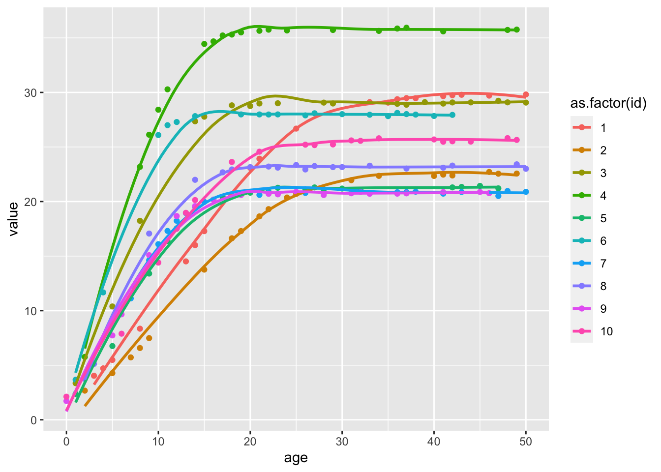
Example of what simulated data looks like
ggplot (bmi %>% filter (id < 11 ), aes (x= age, y= value)) + geom_point (aes (colour= as.factor (id))) + geom_smooth (aes (colour= as.factor (id)), se= FALSE )
`geom_smooth()` using method = 'loess' and formula = 'y ~ x'
Stratifying by age, and getting main effect in each stratum
<- lapply (unique (bmi$ age), function (a) {<- subset (bmi, age == a) %>% slice_sample (n= 1000 )print (dim (x))<- bind_rows (summary (lm (value ~ g1, x))$ coef %>% as_tibble () %>% mutate (g= 1 ) %>% slice_tail (n= 1 ),summary (lm (value ~ g2, x))$ coef %>% as_tibble () %>% mutate (g= 2 ) %>% slice_tail (n= 1 )names (r) <- c ("beta" , "se" , "tval" , "pval" , "g" )$ age <- areturn (r)%>% bind_rows ()
[1] 1000    5
[1] 1000    5
[1] 1000    5
[1] 1000    5
[1] 1000    5
[1] 1000    5
[1] 1000    5
[1] 1000    5
[1] 1000    5
[1] 1000    5
[1] 1000    5
[1] 1000    5
[1] 1000    5
[1] 1000    5
[1] 1000    5
[1] 1000    5
[1] 1000    5
[1] 1000    5
[1] 1000    5
[1] 1000    5
[1] 1000    5
[1] 1000    5
[1] 1000    5
[1] 1000    5
[1] 1000    5
[1] 1000    5
[1] 1000    5
[1] 1000    5
[1] 1000    5
[1] 1000    5
[1] 1000    5
[1] 1000    5
[1] 1000    5
[1] 1000    5
[1] 1000    5
[1] 1000    5
[1] 1000    5
[1] 1000    5
[1] 1000    5
[1] 1000    5
[1] 1000    5
[1] 1000    5
[1] 1000    5
[1] 1000    5
[1] 1000    5
[1] 1000    5
[1] 1000    5
[1] 1000    5
[1] 1000    5
[1] 1000    5
[1] 1000    5
# A tibble: 102 × 6
    beta     se  tval     pval     g   age
   <dbl>  <dbl> <dbl>    <dbl> <dbl> <int>
 1 0.578 0.0753  7.68 3.88e-14     1     3
 2 0.653 0.0750  8.71 1.28e-17     2     3
 3 0.481 0.114   4.21 2.82e- 5     1     4
 4 1.08  0.117   9.17 2.57e-19     2     4
 5 1.13  0.164   6.91 8.44e-12     1     5
 6 1.46  0.163   8.92 2.25e-18     2     5
 7 1.59  0.257   6.17 9.71e-10     1     8
 8 1.67  0.250   6.67 4.32e-11     2     8
 9 2.52  0.286   8.81 5.51e-18     1    13
10 1.40  0.297   4.71 2.85e- 6     2    13
# ℹ 92 more rows
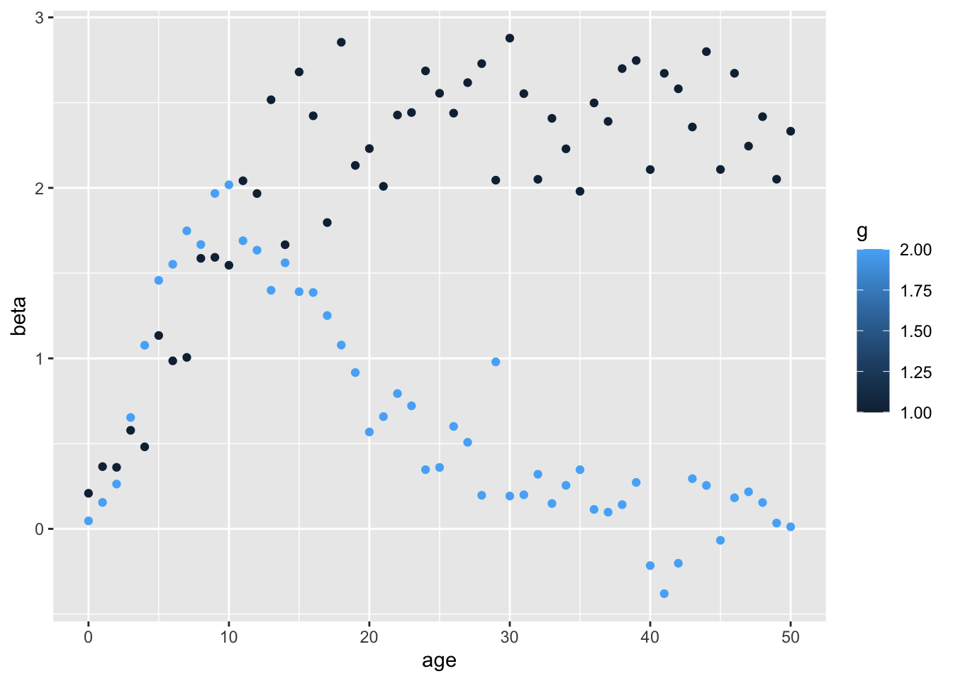
ggplot (o, aes (y= beta, x= age)) + geom_point (aes (colour= g))
Makes sense because g1 influences the asymptote, and g2 influences the rate of growth.
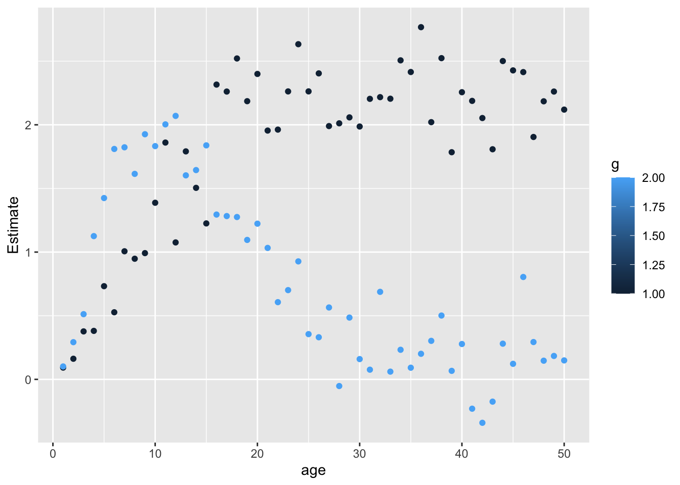
Interaction with main effect - does it give the same thing?
<- bmi %>% group_by (id) %>% slice_sample (n= 1 ) %>% summary (lm (value ~ g1 * as.factor (age), .))$ coef}<- bmi %>% group_by (id) %>% slice_sample (n= 1 ) %>% summary (lm (value ~ g2 * as.factor (age), .))$ coef}<- bind_cols (p = rownames (oi1), oi1) %>% as_tibble %>% filter (grepl ("g1:" , p)) %>% mutate (age= gsub ("g1 \\ :as.factor \\ (age \\ )" , "" , p) %>% as.numeric (), g= 1 )<- bind_cols (p = rownames (oi2), oi2) %>% as_tibble %>% filter (grepl ("g2:" , p)) %>% mutate (age= gsub ("g2 \\ :as.factor \\ (age \\ )" , "" , p) %>% as.numeric (), g= 2 )ggplot (bind_rows (oi1, oi2), aes (y= Estimate, x= age)) + geom_point (aes (colour= g))
Linear model for each individual
<- bmi %>% filter (id %in% 1 : 1000 )<- lmer (value ~ age + (1 + age| id), data= temp)
Warning in checkConv(attr(opt, "derivs"), opt$par, ctrl = control$checkConv, :
Model failed to converge with max|grad| = 0.0579551 (tol = 0.002, component 1)
Warning in checkConv(attr(opt, "derivs"), opt$par, ctrl = control$checkConv, : Model is nearly unidentifiable: very large eigenvalue
 - Rescale variables?
  (Intercept)          age
1 -3.11384947  0.164278524
2 -4.39460900  0.033832734
3  4.75739472 -0.012807851
4 11.70591067  0.013564999
5 -0.06871647 -0.050490788
6  5.65167436 -0.005632972
rbind (summary (lm (b$ id[,1 ] ~ temp$ g1[! duplicated (temp$ id)]))$ coef[2 ,],summary (lm (b$ id[,2 ] ~ temp$ g1[! duplicated (temp$ id)]))$ coef[2 ,],summary (lm (b$ id[,1 ] ~ temp$ g2[! duplicated (temp$ id)]))$ coef[2 ,],summary (lm (b$ id[,2 ] ~ temp$ g2[! duplicated (temp$ id)]))$ coef[2 ,]
        Estimate  Std. Error   t value     Pr(>|t|)
[1,]  1.05784708 0.194558484  5.437168 6.807184e-08
[2,]  0.02622162 0.004303497  6.093097 1.579452e-09
[3,]  1.30851566 0.195321406  6.699295 3.493596e-11
[4,] -0.02265172 0.004374294 -5.178370 2.706779e-07
Summary
Stratifying by age gives same result as fitting age as an interaction - provided that interaction includes main effects for snp and age
Linear model still picks things up
Experiment - interactions with a collider
If there is a binary variable that is a collider, does it make a difference if it is tested stratified or as an interaction term
note this isn’t an issue for age which can’t be a collider
<- 10000 <- rnorm (n)<- rnorm (n)<- x + y + rnorm (n)<- rbinom (n, 1 , plogis (u))summary (lm (y ~ x, subset= C== 1 ))$ coef[2 ,1 ]summary (lm (y ~ x, subset= C== 0 ))$ coef[2 ,1 ]summary (lm (y ~ x))$ coef[2 ,1 ]
summary (lm (y ~ x * as.factor (C)))
Call:
lm(formula = y ~ x * as.factor(C))

Residuals:
    Min      1Q  Median      3Q     Max
-3.6992 -0.6213 -0.0028  0.6146  3.3290

Coefficients:
                Estimate Std. Error t value Pr(>|t|)
(Intercept)     -0.37280    0.01379 -27.034   <2e-16 ***
x               -0.11976    0.01423  -8.415   <2e-16 ***
as.factor(C)1    0.74257    0.01964  37.802   <2e-16 ***
x:as.factor(C)1 -0.00767    0.01993  -0.385      0.7
---
Signif. codes:  0 '***' 0.001 '**' 0.01 '*' 0.05 '.' 0.1 ' ' 1

Residual standard error: 0.9241 on 9996 degrees of freedom
Multiple R-squared:  0.1251,    Adjusted R-squared:  0.1248
F-statistic: 476.5 on 3 and 9996 DF,  p-value: < 2.2e-16
summary (lm (y ~ x : as.factor (C)))
Call:
lm(formula = y ~ x:as.factor(C))

Residuals:
    Min      1Q  Median      3Q     Max
-4.0158 -0.6645 -0.0068  0.6616  3.2348

Coefficients:
                 Estimate Std. Error t value Pr(>|t|)
(Intercept)     -0.006836   0.010499  -0.651    0.515
x:as.factor(C)0  0.009325   0.014769   0.631    0.528
x:as.factor(C)1 -0.001655   0.014488  -0.114    0.909

Residual standard error: 0.988 on 9997 degrees of freedom
Multiple R-squared:  4.045e-05, Adjusted R-squared:  -0.0001596
F-statistic: 0.2022 on 2 and 9997 DF,  p-value: 0.8169
Summary
interaction with a collider is a problem as expected
R version 4.3.0 (2023-04-21)
Platform: aarch64-apple-darwin20 (64-bit)
Running under: macOS Ventura 13.5.2

Matrix products: default
BLAS:   /Library/Frameworks/R.framework/Versions/4.3-arm64/Resources/lib/libRblas.0.dylib
LAPACK: /Library/Frameworks/R.framework/Versions/4.3-arm64/Resources/lib/libRlapack.dylib;  LAPACK version 3.11.0

locale:
[1] en_GB.UTF-8/en_GB.UTF-8/en_GB.UTF-8/C/en_GB.UTF-8/en_GB.UTF-8

time zone: Europe/London
tzcode source: internal

attached base packages:
[1] stats     graphics  grDevices utils     datasets  methods   base

other attached packages:
[1] lme4_1.1-33   Matrix_1.5-4  ggplot2_3.4.2 dplyr_1.1.2

loaded via a namespace (and not attached):
 [1] gtable_0.3.3      jsonlite_1.8.7    compiler_4.3.0    Rcpp_1.0.10
 [5] tidyselect_1.2.0  splines_4.3.0     scales_1.2.1      boot_1.3-28.1
 [9] yaml_2.3.7        fastmap_1.1.1     lattice_0.21-8    R6_2.5.1
[13] labeling_0.4.2    generics_0.1.3    knitr_1.43        htmlwidgets_1.6.2
[17] MASS_7.3-58.4     tibble_3.2.1      nloptr_2.0.3      munsell_0.5.0
[21] minqa_1.2.5       pillar_1.9.0      rlang_1.1.1       utf8_1.2.3
[25] xfun_0.39         cli_3.6.1         mgcv_1.8-42       withr_2.5.0
[29] magrittr_2.0.3    digest_0.6.31     grid_4.3.0        rstudioapi_0.14
[33] lifecycle_1.0.3   nlme_3.1-162      vctrs_0.6.3       evaluate_0.21
[37] glue_1.6.2        farver_2.1.1      fansi_1.0.4       colorspace_2.1-0
[41] rmarkdown_2.22    tools_4.3.0       pkgconfig_2.0.3   htmltools_0.5.5