Logistic regression residuals

Background

Using REML to adjust for pedigree and then taking residuals to estimate PRS association. However the original trait is binary and the residuals are continuous, how to interpret the effect size?

Analysis

Simulate data - a confounder influences x and y, x influences y, and y is binary.

set.seed(1234)
n <- 10000
u <- rnorm(n)
x <- rnorm(n) + u
a <- rnorm(n) + x + u - 1
y <- rbinom(n, 1, plogis(a))
table(y)

y
   0    1 
6331 3669 

Estimate using glm

summary(glm(y ~ x + u, family="binomial"))$coef

              Estimate Std. Error   z value      Pr(>|z|)
(Intercept) -0.8456496 0.02749282 -30.75892 9.290785e-208
x            0.7864091 0.02827687  27.81104 3.189961e-170
u            0.8236558 0.03882063  21.21696 6.659380e-100

Transformation term

mu <- sum(y) / length(y)
tr <- mu * (1-mu)

Get residuals (raw)

yres_raw <- residuals(glm(y ~ u, family="binomial"), type="response")
summary(lm(yres_raw ~ x))$coef

                Estimate  Std. Error     t value     Pr(>|t|)
(Intercept) 9.859144e-05 0.004038968  0.02441006 9.805260e-01
x           6.044366e-02 0.002850011 21.20821889 1.114094e-97

After transformation

lm(yres_raw ~ x)$coef[2] / tr

       x 
0.260214 

Get residuals (deviance)

yres_dev <- residuals(glm(y ~ u, family="binomial"))
summary(lm(yres_dev ~ x))$coef

               Estimate  Std. Error   t value      Pr(>|t|)
(Intercept) -0.06563045 0.009654231 -6.798102  1.120585e-11
x            0.20379274 0.006812301 29.915404 2.104826e-188

After transformation

lm(yres_dev ~ x)$coef[2] / tr

        x 
0.8773415 

Range

library(dplyr)

Attaching package: 'dplyr'

The following objects are masked from 'package:stats':

    filter, lag

The following objects are masked from 'package:base':

    intersect, setdiff, setequal, union

param <- expand.grid(
    b=seq(-1, 1, by=0.1),
    int=seq(-2,0, by=0.2)
)

o <- lapply(1:nrow(param), \(i) {
    u <- rnorm(n)
    x <- rnorm(n) + u
    a <- rnorm(n) + x * param$b[i] + u + param$int[i]
    y <- rbinom(n, 1, plogis(a))
    mu <- sum(y) / length(y)
    tr <- mu * (1-mu)
    bhat <- glm(y ~ x + u, family="binomial")$coef[2]
    yres_raw <- residuals(glm(y ~ u, family="binomial"), type="response")
    bhat_raw <- lm(yres_raw ~ x)$coef[2]
    yres_dev <- residuals(glm(y ~ u, family="binomial"))
    bhat_dev <- lm(yres_dev ~ x)$coef[2]
    tibble(bhat, bhat_raw, bhat_dev, bhat_raw_tr = bhat_raw / tr, bhat_dev_tr=bhat_dev / tr, tr=tr)
}) %>% bind_rows() %>% bind_cols(param, .)

plot

pairs(o %>% select(-c(int, tr)))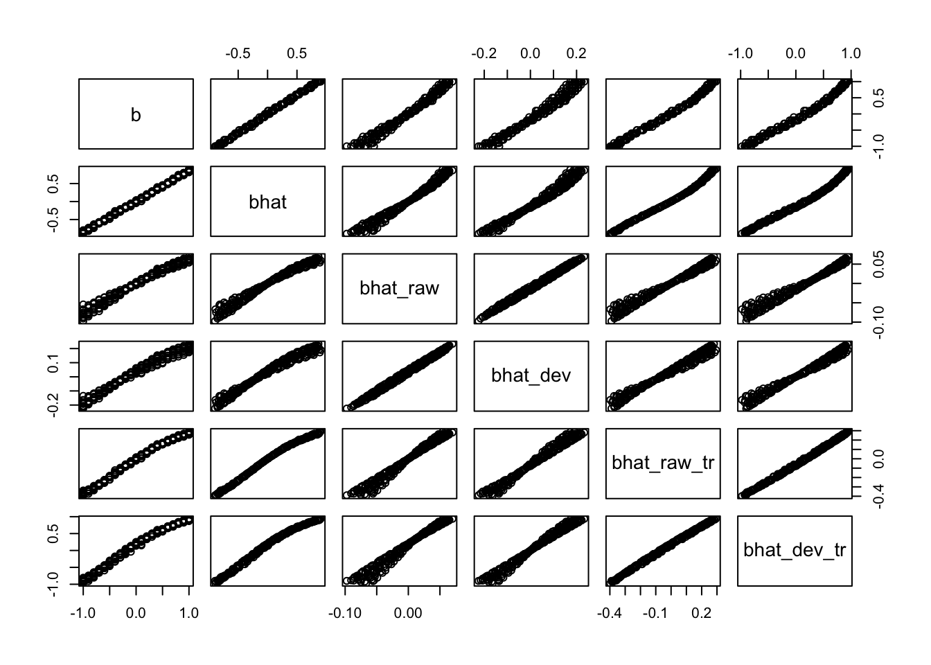

dim(o)

[1] 231   8

Looks like the deviance residuals are on the same scale after transformation, but will need a bit of work to translate between deviance and raw

https://data.library.virginia.edu/understanding-deviance-residuals/

---

sessionInfo()

R version 4.3.0 (2023-04-21)
Platform: aarch64-apple-darwin20 (64-bit)
Running under: macOS Monterey 12.6.8

Matrix products: default
BLAS:   /Library/Frameworks/R.framework/Versions/4.3-arm64/Resources/lib/libRblas.0.dylib 
LAPACK: /Library/Frameworks/R.framework/Versions/4.3-arm64/Resources/lib/libRlapack.dylib;  LAPACK version 3.11.0

locale:
[1] en_US.UTF-8/en_US.UTF-8/en_US.UTF-8/C/en_US.UTF-8/en_US.UTF-8

time zone: Europe/London
tzcode source: internal

attached base packages:
[1] stats     graphics  grDevices utils     datasets  methods   base     

other attached packages:
[1] dplyr_1.1.2

loaded via a namespace (and not attached):
 [1] digest_0.6.31     utf8_1.2.3        R6_2.5.1          fastmap_1.1.1    
 [5] tidyselect_1.2.0  xfun_0.39         magrittr_2.0.3    glue_1.6.2       
 [9] tibble_3.2.1      knitr_1.43        pkgconfig_2.0.3   htmltools_0.5.5  
[13] generics_0.1.3    rmarkdown_2.22    lifecycle_1.0.3   cli_3.6.1        
[17] fansi_1.0.4       vctrs_0.6.2       withr_2.5.0       compiler_4.3.0   
[21] rstudioapi_0.14   tools_4.3.0       pillar_1.9.0      evaluate_0.21    
[25] yaml_2.3.7        rlang_1.1.1       jsonlite_1.8.5    htmlwidgets_1.6.2