MR and imperfect clumping

Background

4000 instruments for educational attainment using clumping r2 = 0.1, and se doubles when using r2 = 0.001.

That smaller standard error is either due to the R2 in the exposure being higher or the non-independence of effects artificially increasing precision, or a mixture of both.

So the question is the impact of the latter – if we have some true correlation structure with realistic F stats at a specific locus, and then we try to clump at r2 = 0.001 vs 0.1, how many instruments do we retain (it should be 1) and if more than 1, what is that impact on the standard error

library(dplyr)

Attaching package: 'dplyr'

The following objects are masked from 'package:stats':

    filter, lag

The following objects are masked from 'package:base':

    intersect, setdiff, setequal, union

library(simulateGP)
library(TwoSampleMR)

TwoSampleMR version 0.5.7 
[>] New: Option to use non-European LD reference panels for clumping etc
[>] Some studies temporarily quarantined to verify effect allele
[>] See news(package='TwoSampleMR') and https://gwas.mrcieu.ac.uk for further details

Attaching package: 'TwoSampleMR'

The following objects are masked from 'package:simulateGP':

    allele_frequency, contingency, get_population_allele_frequency

library(purrr)
library(ggplot2)

Simulate causal snp g + another that is correlated with it

n <- 100000
g <- correlated_binomial(n, p1=0.5, p2=0.5, rho=sqrt(0.1))
# x caused by just snp 1
x <- g[,1] * 0.5 + rnorm(n)
y <- x * 0.5 + rnorm(n)

# MR using both SNPs, treating as if they are independent
get_effs(x, y, g) %>% mr(method="mr_ivw") %>% str

Analysing 'X' on 'Y'

'data.frame':   1 obs. of  9 variables:
 $ id.exposure: chr "X"
 $ id.outcome : chr "Y"
 $ outcome    : chr "Y"
 $ exposure   : chr "X"
 $ method     : chr "Inverse variance weighted"
 $ nsnp       : int 2
 $ b          : num 0.497
 $ se         : num 0.00956
 $ pval       : num 0

# MR using just the causal SNP
get_effs(x, y, g[,1, drop=F]) %>% mr(method=c("mr_ivw", "mr_wald_ratio")) %>% str

Analysing 'X' on 'Y'

'data.frame':   1 obs. of  9 variables:
 $ id.exposure: chr "X"
 $ id.outcome : chr "Y"
 $ outcome    : chr "Y"
 $ exposure   : chr "X"
 $ method     : chr "Wald ratio"
 $ nsnp       : num 1
 $ b          : num 0.496
 $ se         : num 0.0101
 $ pval       : num 0

There’s hardly any difference in the SE here. Try over a range of scenarios

param <- expand.grid(
    r2=seq(0, 1, by=0.02),
    bgx=seq(0,1, by=0.2),
    bxy=seq(0,1, by=0.2),
    n=100000
)
param$sim <- 1:nrow(param)
dim(param)

[1] 1836    5

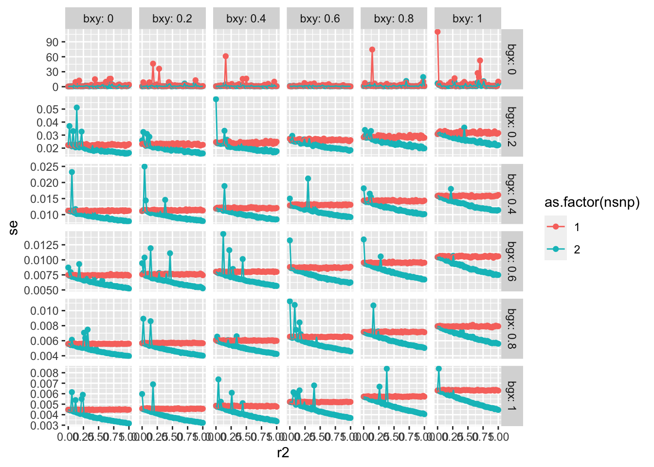
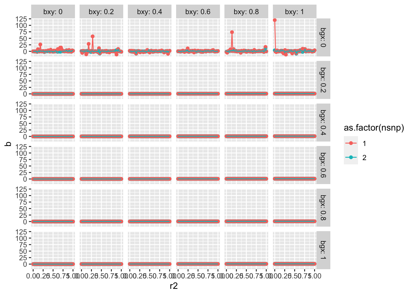
res <- map(1:nrow(param), \(i){
    g <- correlated_binomial(param$n[i], p1=0.5, p2=0.5, rho=sqrt(param$r2[i]))
    # x caused by just snp 1
    x <- g[,1] * param$bgx[i] + rnorm(n)
    y <- x * param$bxy[i] + rnorm(n)

    bind_rows(
        get_effs(x, y, g) %>% {suppressMessages(mr(., method="mr_ivw"))},
        get_effs(x, y, g[,1, drop=F]) %>% {suppressMessages(mr(., method="mr_wald_ratio"))}
    ) %>% mutate(sim=param$sim[i]) %>% return()
}) %>% bind_rows %>% inner_join(param, ., by="sim")

Warning in summary.lm(stats::lm(b_out ~ -1 + b_exp, weights = 1/se_out^2)):
essentially perfect fit: summary may be unreliable

Standard errors across all scenarios

ggplot(res, aes(x=r2, y=se)) +
geom_point(aes(colour=as.factor(nsnp))) +
geom_line(aes(colour=as.factor(nsnp))) +
facet_grid(bgx ~ bxy, labeller=label_both, scale="free_y")

Bias across all scenarios:

ggplot(res, aes(x=r2, y=b)) +
geom_point(aes(colour=as.factor(nsnp))) +
geom_line(aes(colour=as.factor(nsnp))) +
facet_grid(bgx ~ bxy, labeller=label_both)

Look at just one

ggplot(res %>% filter(bgx == 0.2, bxy == 0.2), aes(x=r2, y=se)) +
geom_point(aes(colour=as.factor(nsnp))) +
geom_line(aes(colour=as.factor(nsnp))) +
facet_grid(bgx ~ bxy, labeller=label_both, scale="free_y")

Summary

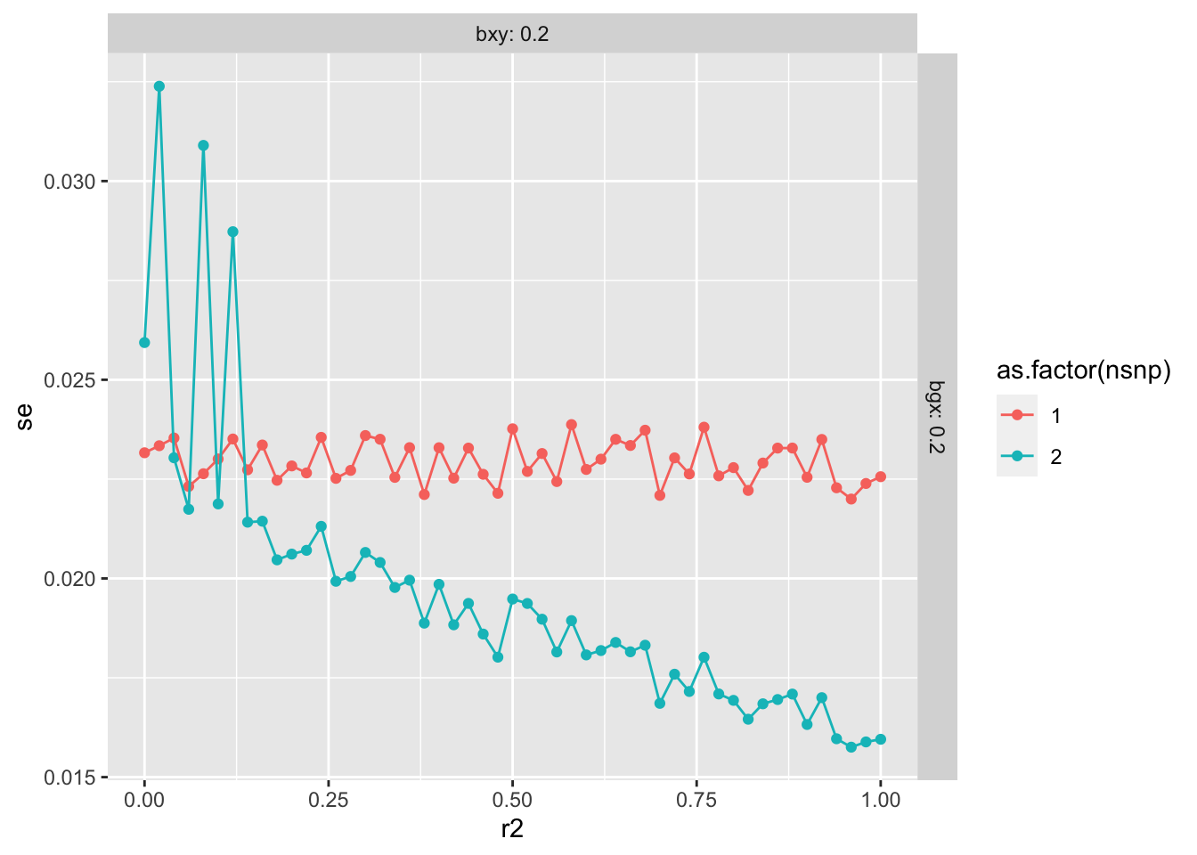
• Relaxed r2 e.g. from 0 to 0.1 doesn’t seem to have a huge impact on standard errors
• In the one SNP situation relaxed r2 has no impact on bias, and could only plausibly change things under substantial heterogeneity which correlates with overrepresentation.
• More realistic simulations would look at whether this changes when the p-value at the second locus is very large, and would also look at the probability of erroneously keeping multiple loci for a single causal variant
• Some instability in SEs when correlated SNPs used

---

sessionInfo()

R version 4.3.0 (2023-04-21)
Platform: aarch64-apple-darwin20 (64-bit)
Running under: macOS Monterey 12.6.2

Matrix products: default
BLAS:   /Library/Frameworks/R.framework/Versions/4.3-arm64/Resources/lib/libRblas.0.dylib 
LAPACK: /Library/Frameworks/R.framework/Versions/4.3-arm64/Resources/lib/libRlapack.dylib;  LAPACK version 3.11.0

locale:
[1] en_US.UTF-8/en_US.UTF-8/en_US.UTF-8/C/en_US.UTF-8/en_US.UTF-8

time zone: Europe/Rome
tzcode source: internal

attached base packages:
[1] stats     graphics  grDevices utils     datasets  methods   base     

other attached packages:
[1] ggplot2_3.4.2     purrr_1.0.1       TwoSampleMR_0.5.7 simulateGP_0.1.2 
[5] dplyr_1.1.2      

loaded via a namespace (and not attached):
 [1] vctrs_0.6.2       cli_3.6.1         knitr_1.43        rlang_1.1.1      
 [5] xfun_0.39         generics_0.1.3    jsonlite_1.8.5    labeling_0.4.2   
 [9] glue_1.6.2        colorspace_2.1-0  plyr_1.8.8        htmltools_0.5.5  
[13] scales_1.2.1      fansi_1.0.4       rmarkdown_2.22    grid_4.3.0       
[17] munsell_0.5.0     evaluate_0.21     tibble_3.2.1      fastmap_1.1.1    
[21] yaml_2.3.7        lifecycle_1.0.3   compiler_4.3.0    Rcpp_1.0.10      
[25] htmlwidgets_1.6.2 pkgconfig_2.0.3   rstudioapi_0.14   farver_2.1.1     
[29] digest_0.6.31     R6_2.5.1          tidyselect_1.2.0  utf8_1.2.3       
[33] pillar_1.9.0      magrittr_2.0.3    withr_2.5.0       gtable_0.3.3     
[37] tools_4.3.0