Confounder instruments via networks

confounding
mr
Author

Gibran Hemani

Published

July 7, 2023

Background

In a previous post looked at the rate of bias as GWAS sample size increases. It was predicated on smaller effects more likely acting via confounders.

What is the justification for smaller effects acting via confounders? After all, all effects likely act via mediators. Some of those mediators will confound a X-Y relationship while some will not. Is there any reason to believe that as effects get smaller they’re more likely to act via a confounder?

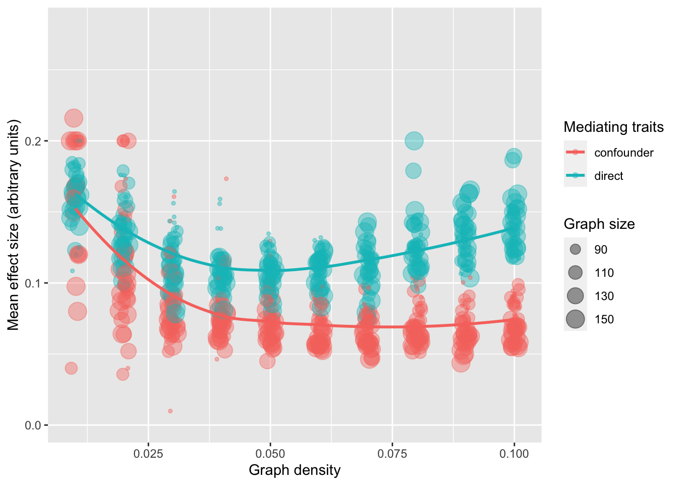
Imagine a large DAG representing the genotype-phenotype map. All nodes that have no parents are genetic variants. All other nodes are traits. If you choose any two traits, one as the exposure and one as the outcome, what is the nature of the instruments for the exposure? Hypothesis: the instruments that are mediated by confounders are likely to be more distal from the exposure, compared to those that act via non-confounding mediators.

These simulations aim to test that.

library(dagitty)
library(dplyr)

Attaching package: 'dplyr'
The following objects are masked from 'package:stats':

    filter, lag
The following objects are masked from 'package:base':

    intersect, setdiff, setequal, union
library(furrr)
Loading required package: future
library(ggplot2)
library(tictoc)

simulategraphconf <- function(n, p) {
    # Generate graph
    g <- dagitty::randomDAG(n, p)

    # All ancestors
    anc <- lapply(names(g), \(x) ancestors(g, x))
    names(anc) <- names(g)

    # Identify genetic factors (no ancestors)
    temp <- lapply(anc, length)
    temp <- tibble(node=names(temp), nanc=unlist(temp))

    gen <- subset(temp, nanc==1)$node
    message("Number of genetic variants: ", length(gen))

    traits <- subset(temp, nanc != 1)$node
    message("Number of traits: ", length(traits))
    # Find distance of all genetic variants to 

    # Find all trait pairs
    tp <- lapply(traits, \(tr) {
        temp <- ancestors(g, tr)
        tibble(x=temp, y=tr) %>%
            filter(! x %in% c(gen, tr))
    }) %>% bind_rows
    # tp <- expand.grid(x=traits, y=traits) %>%
    #   as_tibble() %>%
    #   filter(x != y)
    message("Number of trait pairs: ", nrow(tp))

    res <- furrr::future_map(1:min(nrow(tp), 500), \(i)
    {
        x_ancestors <- ancestors(g, tp$x[i])
        x_ancestors <- x_ancestors[x_ancestors %in% gen]
        y_ancestors <- ancestors(g, tp$y[i])
        y_ancestors <- y_ancestors[y_ancestors %in% gen]

        conf <- c()
        nonconf <- c()
        for(a in y_ancestors)
        {
            x <- paths(g, a, tp$y[i], dir=T)$paths
            if(any(!grepl(paste0(" ", tp$x[i], " "), x)))
            {
                conf <- c(conf, a)
            } else {
                nonconf <- c(nonconf, a)
            }
        }
        bind_rows(
            lapply(conf, function(co)
            {
                pa <- paths(g, co, tp$x[i], directed=TRUE)$paths
                if(length(pa) != 0)
                {
                    tibble(
                        x=tp$x[i],
                        y=tp$y[i],
                        gen=co,
                        type="confounder",
                        w=pa %>%
                            sapply(., function(x)
                            {
                                stringr::str_count(x, "->") %>%
                                unlist() %>%
                                {0.2^.}
                            }) %>% sum
                    )
                } else {
                    NULL
                }
            }) %>% bind_rows(),
            lapply(nonconf, function(co)
            {
                pa <- paths(g, co, tp$x[i], directed=TRUE)$paths
                if(length(pa) != 0)
                {
                    tibble(
                        x=tp$x[i],
                        y=tp$y[i],
                        gen=co,
                        type="direct",
                        w=pa %>%
                            sapply(., function(x)
                            {
                                stringr::str_count(x, "->") %>%
                                unlist() %>%
                                {0.2^.}
                            }) %>% sum
                    )
                } else {
                    NULL
                }
            }) %>% bind_rows()
        )
    }) %>% bind_rows()
    # res$causal <- paste(res$x, res$y) %in% paste(tpc$x, tpc$y)
    return(res)
}

set.seed(1234) # note this doesn't work for dagitty - for seed should use pcalg
plan(multisession, workers=1)
tic()
res <- simulategraphconf(50, 0.1)
Number of genetic variants: 13
Number of traits: 37
Number of trait pairs: 191
toc()
16.505 sec elapsed
res %>% group_by(type) %>% summarise(
    n=n(),
    w=mean(w)
)
# A tibble: 2 × 3
  type           n      w
  <chr>      <int>  <dbl>
1 confounder   310 0.0882
2 direct       190 0.120 

Run the simulations (note, ran this externally on epifranklin)

param <- expand.grid(
    n=seq(75, 150, by=25),
    p=seq(0.01, 0.1, by=0.01),
    rep=c(1:10)
)

res <- lapply(1:nrow(param), \(i) {
    message(i)
    res <- simulategraphconf(param$n[i], param$p[i])
    res %>% group_by(type) %>% summarise(
        ntype=n(),
        w=mean(w)
    ) %>% mutate(
        n=param$n[i],
        p=param$p[i],
        rep=param$rep[i]
    )
}) %>% bind_rows(res)
res <- readRDS("mrnetworkconf.rds")
res %>%
ggplot(., aes(x=p, y=w)) +
geom_jitter(aes(colour=type, size=n), alpha=0.4, width=0.001) +
geom_smooth(aes(colour=type), se=F) +
labs(size="Graph size", x="Graph density", y="Mean effect size (arbitrary units)", colour="Mediating traits")
`geom_smooth()` using method = 'loess' and formula = 'y ~ x'
Warning: Removed 594 rows containing non-finite values (`stat_smooth()`).
Warning: Removed 594 rows containing missing values (`geom_point()`).

So the effect sizes for instruments acting via non-confounders tend to be substantially larger than those acting via confounders.

ggsave("mrnetworkconf.pdf")
Saving 7 x 5 in image
`geom_smooth()` using method = 'loess' and formula = 'y ~ x'
Warning: Removed 594 rows containing non-finite values (`stat_smooth()`).
Warning: Removed 594 rows containing missing values (`geom_point()`).

Alternative graph generating method

Phenomic layers. But it’s not clear how to generate this realistically. Not implemented in sims yet.

sim_graph <- function(ng, ne, np, nm, nd, nge, nep, npm, nmd) {
    links <- bind_rows(
        tibble(
            x=sample(paste0("g", 1:ng), nge, replace=TRUE),
            y=sample(paste0("e", 1:ne), nge, replace=TRUE)
        ),
        tibble(
            x=sample(paste0("e", 1:ne), nep, replace=TRUE),
            y=sample(paste0("p", 1:np), nep, replace=TRUE)
        ),
        tibble(
            x=sample(paste0("p", 1:np), npm, replace=TRUE),
            y=sample(paste0("m", 1:nm), npm, replace=TRUE)
        ),
        tibble(
            x=sample(paste0("m", 1:nm), nmd, replace=TRUE),
            y=sample(paste0("d", 1:nd), nmd, replace=TRUE)
        )
    ) %>% mutate(
        rel=paste0(x, " -> ", y)
    )
    g <- dagitty(paste("dag{",
        paste(links$rel, collapse="\n"),
    "}"))
    return(g)
}

g <- sim_graph(400, 200, 300, 400, 20, 600, 200, 200, 300)
plot(g)
Plot coordinates for graph not supplied! Generating coordinates, see ?coordinates for how to set your own.
Warning in arrows(ax1[directed], -ay1[directed], ax2[directed], -ay2[directed],
: zero-length arrow is of indeterminate angle and so skipped

ancestors(g, "d1") %>% {grep("g", ., value=TRUE)}
[1] "g79"  "g341" "g262" "g199" "g186" "g93"  "g170"
paths(g, "g79", "d1", dir=T)
$paths
[1] "g79 -> e43 -> p236 -> m215 -> d1"

$open
[1] TRUE
paths(g, "g79", "d3", dir=T)
$paths
list()

$open
list()

Meta regression using exposure effect size

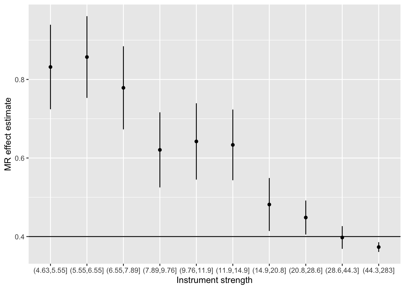
  1. Simulate individual level data in system in which u causes x and y, and both x and u have independent instruments
  2. Identify instruments (should include many gx and some gu)
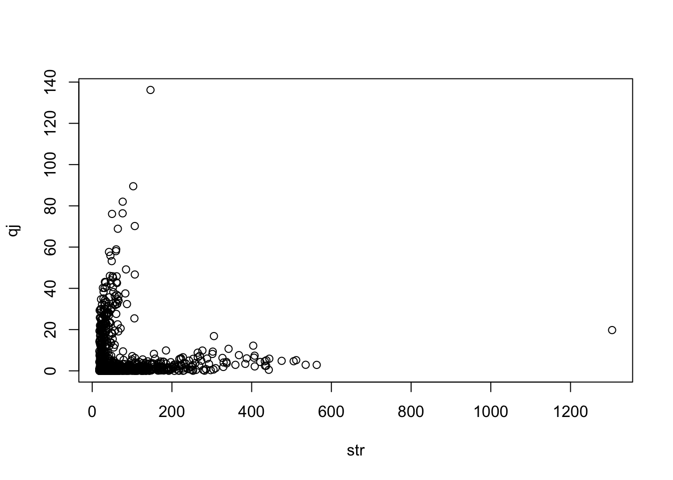
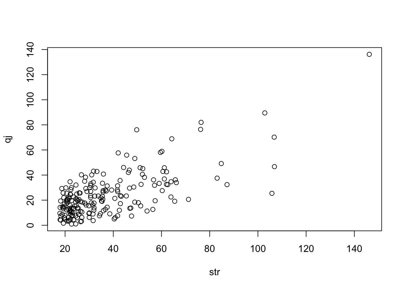
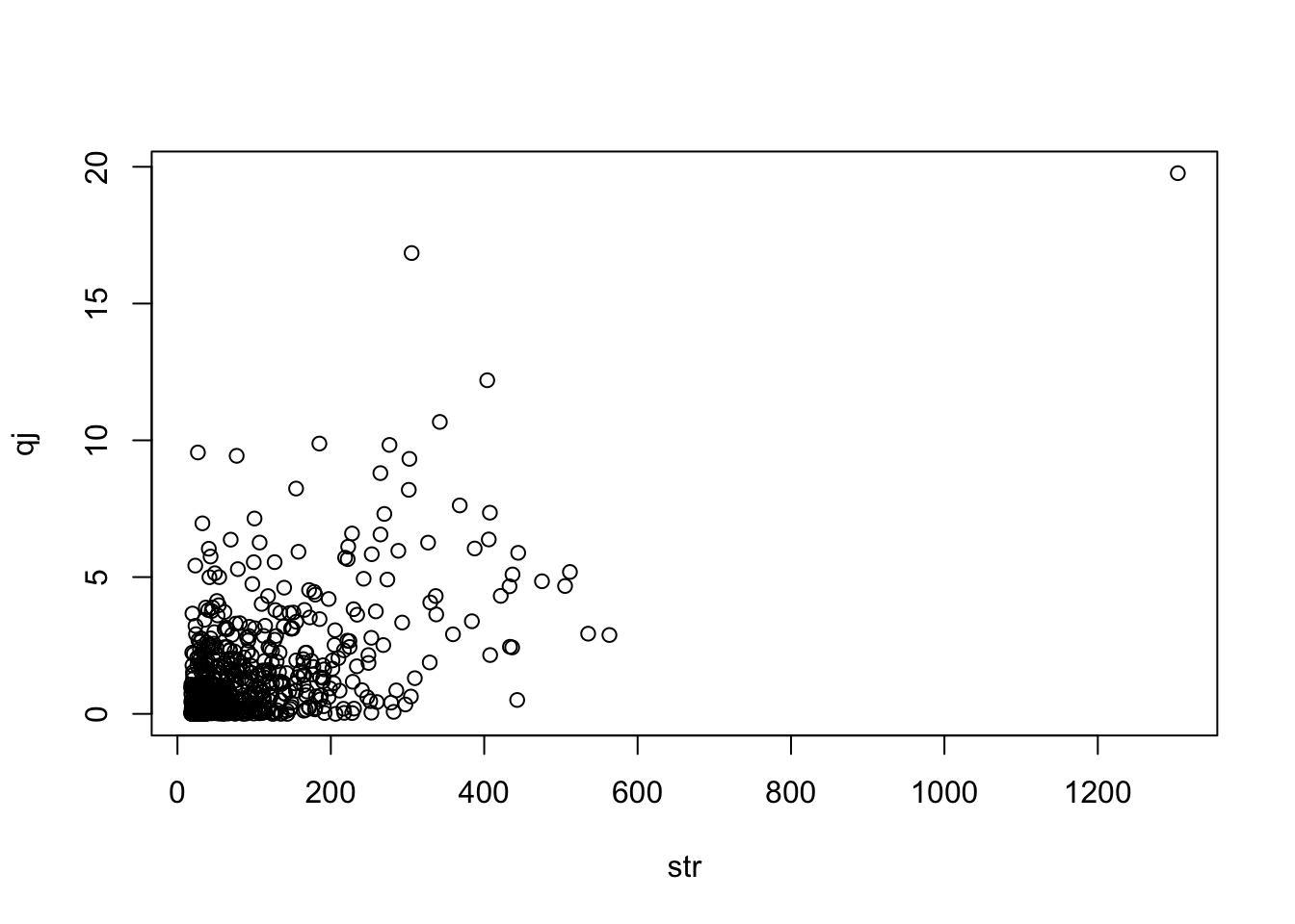
  3. Estimate heterogeneity contribution from each instrument
  4. Meta regression of instrument strength against heterogeneity
library(simulateGP)
library(TwoSampleMR)
TwoSampleMR version 0.5.7 
[>] New: Option to use non-European LD reference panels for clumping etc
[>] Some studies temporarily quarantined to verify effect allele
[>] See news(package='TwoSampleMR') and https://gwas.mrcieu.ac.uk for further details

Attaching package: 'TwoSampleMR'
The following objects are masked from 'package:simulateGP':

    allele_frequency, contingency, get_population_allele_frequency
# 1. simulate system
nid <- 100000
nsnp <- 1000
gx <- make_geno(nid, nsnp, 0.4)
gu <- make_geno(nid, nsnp, 0.4)
bx <- choose_effects(nsnp, sqrt(0.4))
bu <- choose_effects(nsnp, sqrt(0.4))
u <- make_phen(bu, gu)
x <- make_phen(c(bx, 0.4), cbind(gx, u))
y <- make_phen(c(0.4, 0.4), cbind(x, u))
# 2. Identify instruments
dat <- get_effs(x, y, cbind(gx, gu))
dats <- subset(dat, pval.exposure < (0.05/2000))
str(dat)
tibble [2,000 × 18] (S3: tbl_df/tbl/data.frame)
 $ SNP                : int [1:2000] 1 2 3 4 5 6 7 8 9 10 ...
 $ exposure           : chr [1:2000] "X" "X" "X" "X" ...
 $ id.exposure        : chr [1:2000] "X" "X" "X" "X" ...
 $ outcome            : chr [1:2000] "Y" "Y" "Y" "Y" ...
 $ id.outcome         : chr [1:2000] "Y" "Y" "Y" "Y" ...
 $ beta.exposure      : num [1:2000] -0.0368 0.0252 0.0335 -0.0272 0.0328 ...
 $ beta.outcome       : num [1:2000] -0.0185 0.00598 0.01851 -0.00805 0.00889 ...
 $ se.exposure        : num [1:2000] 0.00456 0.00457 0.00456 0.00457 0.00455 ...
 $ se.outcome         : num [1:2000] 0.00456 0.00457 0.00456 0.00457 0.00455 ...
 $ pval.exposure      : num [1:2000] 6.98e-16 3.51e-08 2.07e-13 2.48e-09 5.95e-13 ...
 $ pval.outcome       : num [1:2000] 5.03e-05 1.91e-01 5.01e-05 7.81e-02 5.09e-02 ...
 $ samplesize.exposure: num [1:2000] 1e+05 1e+05 1e+05 1e+05 1e+05 1e+05 1e+05 1e+05 1e+05 1e+05 ...
 $ samplesize.outcome : num [1:2000] 1e+05 1e+05 1e+05 1e+05 1e+05 1e+05 1e+05 1e+05 1e+05 1e+05 ...
 $ units.exposure     : chr [1:2000] "SD" "SD" "SD" "SD" ...
 $ units.outcome      : chr [1:2000] "SD" "SD" "SD" "SD" ...
 $ rsq.exposure       : num [1:2000] 0.000651 0.000304 0.000539 0.000355 0.000519 ...
 $ rsq.outcome        : num [1:2000] 1.64e-04 1.71e-05 1.64e-04 3.10e-05 3.81e-05 ...
 $ mr_keep            : logi [1:2000] TRUE TRUE TRUE TRUE TRUE TRUE ...
table(dats$SNP > 1000)

FALSE  TRUE 
  592   203 
dats$strength <- cut(-log10(dats$pval.exposure), breaks=quantile(-log10(dats$pval.exposure), probs=seq(0, 1, 0.1)))
table(dats$strength)

(4.63,5.55] (5.55,6.55] (6.55,7.89] (7.89,9.76] (9.76,11.9] (11.9,14.9] 
         79          79          80          79          80          79 
(14.9,20.8] (20.8,28.6] (28.6,44.3]  (44.3,283] 
         79          80          79          80 
# Overall MR estimate
res <- mr(dats, method="mr_ivw")
Analysing 'X' on 'Y'
res
  id.exposure id.outcome outcome exposure                    method nsnp
1           X          Y       Y        X Inverse variance weighted  795
          b        se pval
1 0.4757469 0.0102651    0

Stratify by instrument strength

dats %>% group_by(strength) %>% do({mr(., method="mr_ivw")}) %>% 
    ggplot(., aes(x=strength, y=b)) +
    geom_point() +
    geom_errorbar(aes(ymin=b-se*1.96, ymax=b+se*1.96), width=0) +
    geom_hline(yintercept=0.4) +
    labs(x="Instrument strength", y="MR effect estimate")
Analysing 'X' on 'Y'

# 3. Estimate heterogeneity
ss <- mr_singlesnp(dats) %>% filter(!grepl("All", SNP)) %>% mutate(SNP = as.numeric(SNP))
ss$qj <- (1/ss$se^2) * (res$b - ss$b)^2
ss$str <- (dats$beta.exposure/dats$se.exposure)^2
ss$str2 <- -log10(dats$pval.exposure)
mr_heterogeneity(dats, method="mr_ivw")$Q == sum(ss$qj)
[1] TRUE
  1. Meta regression
# All SNPs
summary(lm(qj ~ str, data=ss))

Call:
lm(formula = qj ~ str, data = ss)

Residuals:
    Min      1Q  Median      3Q     Max 
 -8.171  -7.145  -5.373   1.080 129.726 

Coefficients:
             Estimate Std. Error t value Pr(>|t|)    
(Intercept)  8.416813   0.626477  13.435  < 2e-16 ***
str         -0.013380   0.004787  -2.795  0.00531 ** 
---
Signif. codes:  0 '***' 0.001 '**' 0.01 '*' 0.05 '.' 0.1 ' ' 1

Residual standard error: 13.21 on 793 degrees of freedom
Multiple R-squared:  0.009757,  Adjusted R-squared:  0.008508 
F-statistic: 7.813 on 1 and 793 DF,  p-value: 0.005312

Higher strength means lower heterogeneity

# Only x snps
summary(lm(qj ~ str, data=subset(ss, SNP <= 1000)))

Call:
lm(formula = qj ~ str, data = subset(ss, SNP <= 1000))

Residuals:
    Min      1Q  Median      3Q     Max 
-4.8033 -0.8923 -0.4404  0.6002 13.0460 

Coefficients:
             Estimate Std. Error t value Pr(>|t|)    
(Intercept) 0.4515093  0.1019608   4.428 1.13e-05 ***
str         0.0109704  0.0006811  16.106  < 2e-16 ***
---
Signif. codes:  0 '***' 0.001 '**' 0.01 '*' 0.05 '.' 0.1 ' ' 1

Residual standard error: 1.784 on 590 degrees of freedom
Multiple R-squared:  0.3054,    Adjusted R-squared:  0.3042 
F-statistic: 259.4 on 1 and 590 DF,  p-value: < 2.2e-16

Wouldn’t expect this - weaker SNPs should contribute more heterogeneity due to weak instrument bias

summary
function (object, ...) 
UseMethod("summary")
<bytecode: 0x12d4ab510>
<environment: namespace:base>
# Only u snps
summary(lm(qj ~ str, data=subset(ss, SNP > 1000)))

Call:
lm(formula = qj ~ str, data = subset(ss, SNP > 1000))

Residuals:
    Min      1Q  Median      3Q     Max 
-41.201  -8.024  -0.785   7.060  44.492 

Coefficients:
            Estimate Std. Error t value Pr(>|t|)    
(Intercept)  0.99448    1.89762   0.524    0.601    
str          0.62044    0.04559  13.609   <2e-16 ***
---
Signif. codes:  0 '***' 0.001 '**' 0.01 '*' 0.05 '.' 0.1 ' ' 1

Residual standard error: 12.75 on 201 degrees of freedom
Multiple R-squared:  0.4796,    Adjusted R-squared:  0.477 
F-statistic: 185.2 on 1 and 201 DF,  p-value: < 2.2e-16
plot(qj ~ str, ss)

plot(qj ~ str, ss %>% filter(SNP > 1000))

plot(qj ~ str, ss %>% filter(SNP <= 1000))


sessionInfo()
R version 4.3.0 (2023-04-21)
Platform: aarch64-apple-darwin20 (64-bit)
Running under: macOS Monterey 12.6.2

Matrix products: default
BLAS:   /Library/Frameworks/R.framework/Versions/4.3-arm64/Resources/lib/libRblas.0.dylib 
LAPACK: /Library/Frameworks/R.framework/Versions/4.3-arm64/Resources/lib/libRlapack.dylib;  LAPACK version 3.11.0

locale:
[1] en_GB.UTF-8/en_GB.UTF-8/en_GB.UTF-8/C/en_GB.UTF-8/en_GB.UTF-8

time zone: Europe/London
tzcode source: internal

attached base packages:
[1] stats     graphics  grDevices utils     datasets  methods   base     

other attached packages:
[1] TwoSampleMR_0.5.7 simulateGP_0.1.2  purrr_1.0.1       tictoc_1.2       
[5] ggplot2_3.4.2     furrr_0.3.1       future_1.33.0     dplyr_1.1.2      
[9] dagitty_0.3-1    

loaded via a namespace (and not attached):
 [1] utf8_1.2.3        generics_0.1.3    stringi_1.7.12    lattice_0.21-8   
 [5] listenv_0.9.0     digest_0.6.31     magrittr_2.0.3    evaluate_0.21    
 [9] grid_4.3.0        fastmap_1.1.1     plyr_1.8.8        Matrix_1.5-4     
[13] jsonlite_1.8.5    mgcv_1.8-42       fansi_1.0.4       scales_1.2.1     
[17] textshaping_0.3.6 codetools_0.2-19  cli_3.6.1         rlang_1.1.1      
[21] parallelly_1.36.0 munsell_0.5.0     splines_4.3.0     withr_2.5.0      
[25] yaml_2.3.7        tools_4.3.0       parallel_4.3.0    colorspace_2.1-0 
[29] boot_1.3-28.1     globals_0.16.2    curl_5.0.0        vctrs_0.6.2      
[33] R6_2.5.1          lifecycle_1.0.3   stringr_1.5.0     V8_4.3.2         
[37] htmlwidgets_1.6.2 MASS_7.3-58.4     ragg_1.2.5        pkgconfig_2.0.3  
[41] pillar_1.9.0      gtable_0.3.3      glue_1.6.2        Rcpp_1.0.10      
[45] systemfonts_1.0.4 xfun_0.39         tibble_3.2.1      tidyselect_1.2.0 
[49] rstudioapi_0.14   knitr_1.43        farver_2.1.1      htmltools_0.5.5  
[53] nlme_3.1-162      labeling_0.4.2    rmarkdown_2.22    compiler_4.3.0