Latest PRS for height explains ~40% of the variance. Heritability ~0.7. Height has a negative association with coronary heart disease. Height is fixed after adolescence, which means it can only be influenced by a) genetic factors; b) early life exposures; c) stochasticity.
Question: Is the influence of height on CHD different when the modifier is genetic vs non-genetic?
Analysis: Estimate the association of height PRS on CHD, and then residualise height for the PRS and determine the residual height association with CHD.
Model
Gene environment equivalence
Under gene-environment equivalence, the following model:
\[
y_i = \alpha + \beta_{xy} x_i + \epsilon_i
\]
where \(y_i\) is the outcome (e.g. CHD), \(\beta_{xy}\) is the causal effect of the exposure on the outcome and
\[
x_i = a + \sqrt{h^2} g_i + \sqrt{1-h^2} e_i
\]
where \(x_i\) is the exposure (height) in the \(i\)th individual, \(h^2\) is the heritability of height, \(g_i\) is the (perfectly measured) genetic value for individual \(i\) and \(e_i\) is the non-genetic component of height. There is no confounding in this simple model. What is the expected association of g on y?
So this is expected and the basic result for MR. What is the expected association of x on y after it has been residualised for g? First get the residual assuming perfect information of \(g\)
The following objects are masked from 'package:stats':

    filter, lag
The following objects are masked from 'package:base':

    intersect, setdiff, setequal, union
library(ggplot2)n <-100000bxy <-0.3h2 <-0.7g <-rnorm(n)e <-rnorm(n)x <-sqrt(h2) * g +sqrt(1-h2) * ey <- x * bxy +rnorm(n)
Get residual
xres <-residuals(lm(x ~ g)) # simxres_exp <-sqrt(1-h2) * e # expected# check they're the samecor(xres, xres_exp)
[1] 0.9999938
lm(xres ~ xres_exp)$coef[2]
 xres_exp
0.9999876
Assoc of x on y should be
lm(y ~ x)$coef[2] # sim
        x
0.3002834
bxy # expected
[1] 0.3
Expected assoc of g on y
lm(y ~ g)$coef[2] # sim
        g
0.2523371
sqrt(h2)*bxy # expected
[1] 0.250998
Expected assoc of residual x on y
lm(y ~ xres)$coef[2] # sim
     xres
0.2988134
bxy
[1] 0.3
Gene environment non-equivalence
n <-100000bg <-0.3be <-0.6h2 <-0.7g <-rnorm(n)e <-rnorm(n)x <-sqrt(h2) * g +sqrt(1-h2) * ey <- g * bg + e * be +rnorm(n)
Get residual
xres <-residuals(lm(x ~ g)) # simxres_exp <-sqrt(1-h2) * e # expected# check they're the samecor(xres, xres_exp)
[1] 0.9999998
lm(xres ~ xres_exp)$coef[2]
 xres_exp
0.9999996
Association of xres and y
lm(y ~ xres)$coef[2] # sim
    xres
1.086526
be /sqrt(1-h2)
[1] 1.095445
Assoc of x and y - simulation
lm(y ~ x)$coef[2] # sim
        x
0.5760577
bg *sqrt(h2) + be *sqrt(1-h2) # exp
[1] 0.5796315
Incomplete adjustment of g
Does incomplete adjustment of g change things much?
Gene environment equivalence
n <-100000bxy <-0.3h2 <-0.7g_exp <-0.5# proportion of g explained by prsg_explained <-rnorm(n) *sqrt(g_exp)g_unexplained <-rnorm(n) *sqrt(1-g_exp)g <- g_explained + g_unexplainede <-rnorm(n)x <-sqrt(h2) * g +sqrt(1-h2) * ey <- x * bxy +rnorm(n)
Get residual - now this is different from expected above due to residual including some unadjusted genetic variance, but linearly still related
xres <-residuals(lm(x ~ g_explained)) # simxres_exp <-sqrt(1-h2) * e # expected# check they're the samecor(xres, xres_exp)
[1] 0.6786454
lm(xres ~ xres_exp)$coef[2]
xres_exp
1.001644
What is the PRS (explained g) assoc with y?
lm(y ~ g_explained)$coef[2]
g_explained
  0.2557102
Assoc of height with y
lm(y ~ x)$coef[2]
        x
0.3021427
And residual with y
lm(y ~ xres)$coef[2]
     xres
0.3004327
So the residual x effect remains identical to the raw effect of x.
In progress… (ignore for now)
Does confounding change things much?
n <-100000bxy <-0.3bu <-0.3h2 <-0.7u <-rnorm(n)g <-rnorm(n)e <-rnorm(n)x <-sqrt(h2) * g +sqrt(1-h2) * e + u * buy <- x * bxy +rnorm(n) + u * bu
y ~ x
lm(y ~ x)$coef[2]
        x
0.3807293
y ~ x_res
xres <-residuals(lm(x ~ g)) # simxres_exp <-sqrt(1-h2) * e # expected# check they're the samecor(xres, xres_exp)
n <-100000bxy <--0.3h2 <-0.7g <-rnorm(n)e <-rnorm(n)x <-sqrt(h2) * g +sqrt(1-h2) * ey <- x * bxy +rnorm(n)testdat(y, x, g)
# A tibble: 3 × 2
  model      beta
  <chr>     <dbl>
1 y ~ x    -0.306
2 y ~ g    -0.256
3 y ~ xres -0.300
n <-100000buy <-0.3bux <--0.3bxy <-0.3h2 <-0.7u <-rnorm(n)g <-rnorm(n)e <-rnorm(n)x <-sqrt(h2) * g +sqrt(1-h2) * e + bux * uy <- x * bxy +rnorm(n) + buy * utestdat(y, x, g)
# A tibble: 3 × 2
  model      beta
  <chr>     <dbl>
1 y ~ x    0.217
2 y ~ g    0.254
3 y ~ xres 0.0633
n <-100000buy <-0.3bux <--0.3bg <--0.2be <--0.3h2 <-0.7u <-rnorm(n)g <-rnorm(n)e <-rnorm(n)x <-sqrt(h2) * g +sqrt(1-h2) * e + bux * uy <- g * bg + e * be +rnorm(n) + buy * utestdat(y, x, g)
# A tibble: 3 × 2
  model      beta
  <chr>     <dbl>
1 y ~ x    -0.392
2 y ~ g    -0.205
3 y ~ xres -0.655
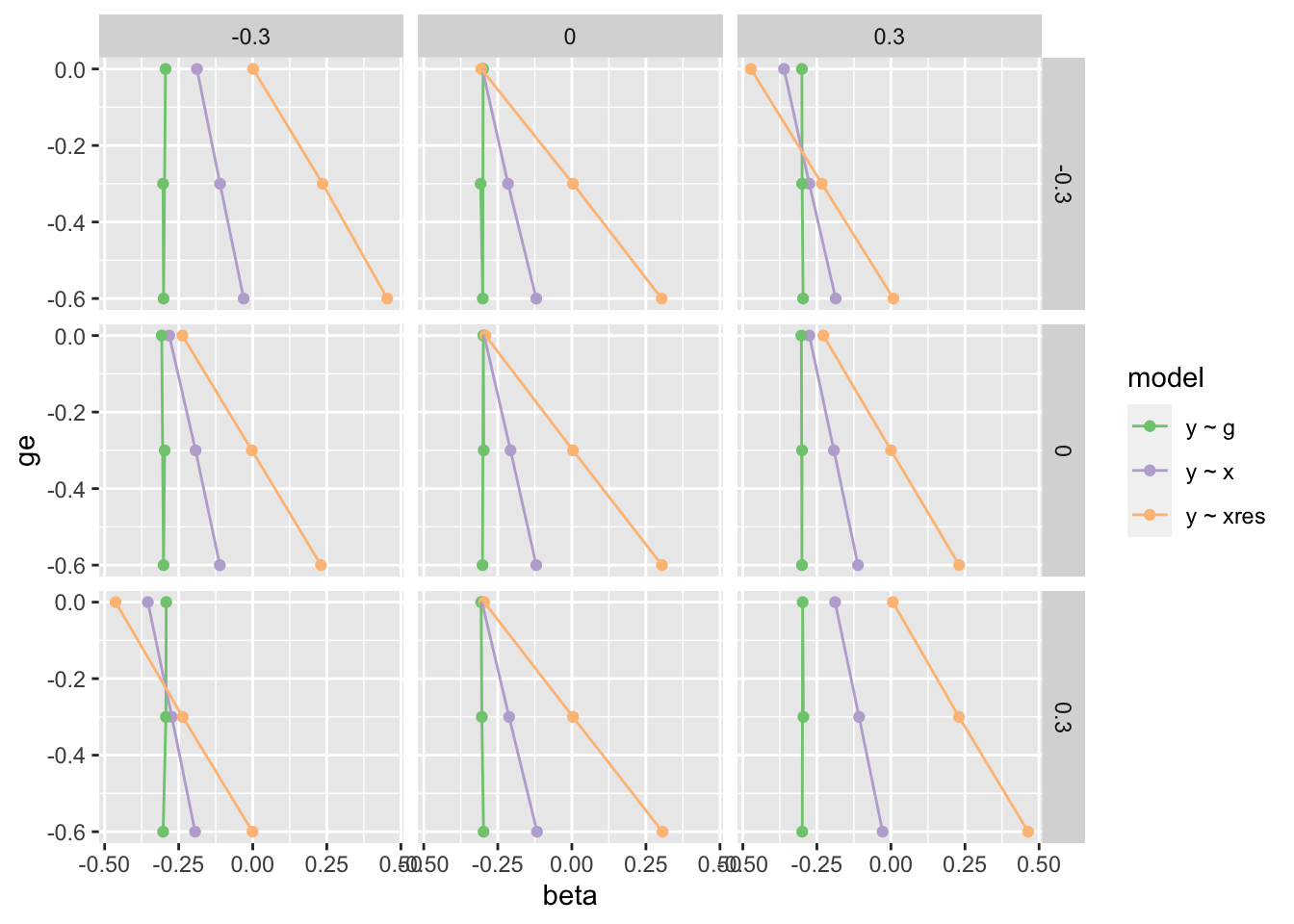
param <-expand.grid(buy =seq(-0.3, 0.3, by=0.3),bux =seq(-0.3, 0.3, by=0.3),bg =seq(-0.3, 0.3, by=0.3),be =seq(-0.3, 0.3, by=0.3))res <-lapply(1:nrow(param), function(i) { n <-100000 buy <- param$buy[i] bux <- param$bux[i] bg <- param$bg[i] be <- param$be[i] h2 <-0.7 u <-rnorm(n) g <-rnorm(n, sd=sqrt(h2)) e <-rnorm(n, sd=sqrt(1-h2)) x <- g + e + bux * u y <- g * bg + e * be +rnorm(n) + buy * utestdat(y, x, g) %>%bind_cols(param[i,])})res <-bind_rows(res)
n <-100000buy <-0bux <-0bg <--0.4be <--0.2h2 <-0.5u <-rnorm(n)g <-rnorm(n, sd=sqrt(h2))e <-rnorm(n, sd=sqrt(1-h2))x <- g + ey <- g * bg + e * be +rnorm(n)testdat(y, x, g)
# A tibble: 3 × 2
  model      beta
  <chr>     <dbl>
1 y ~ x    -0.301
2 y ~ g    -0.397
3 y ~ xres -0.205