Background
Is it possible to convert BF to beta and standard error? According to Giambartolomei et al 2014 -
\[
ABF = \sqrt{1-r} \times exp(rZ^2/2)
\]
so
\[
|Z| = \sqrt{\frac{2 * log(ABF) - log(\sqrt{1-r})}{r}}
\]
here \(r = W / V\) where V is the variance of the SNP effect estimate
\[
V \approx \frac{1}{2np(1-p)}
\]
where n is sample size and p is allele frequency (assumes small amount of variance explained in trait and sd of trait is 1).
Run simulation
Use regional LD matrix to generate summary statistics with a single causal variant
Use SuSiE to perform fine mapping
Convert SuSiE Bayes Factors into Z scores, betas, standard errors
Compare converted Z, beta, se against original simulated Z, beta, SE
Simulation
Libraries
library (simulateGP)library (susieR)library (here)
here() starts at /Users/gh13047/repo/lab-book
Attaching package: 'dplyr'
The following objects are masked from 'package:stats':

    filter, lag
The following objects are masked from 'package:base':

    intersect, setdiff, setequal, union
Conversion function for logBF to z, beta, se
#' Convert log Bayes Factor to summary stats #' #' @param lbf p-vector of log Bayes Factors for each SNP #' @param n Overall sample size #' @param af p-vector of allele frequencies for each SNP #' @param prior_v Variance of prior distribution. SuSiE uses 50 #' #' @return tibble with lbf, af, beta, se, z <- function (lbf, n, af, prior_v= 50 )= sqrt (1 / (2 * n * af * (1 - af)))= prior_v / (prior_v + se^ 2 )= sqrt ((2 * lbf - log (sqrt (1 - r)))/ r)<- z * sereturn (tibble (lbf, af, z, beta, se))
Read in example LD matrix from simulateGP repository
<- readRDS (url ("https://github.com/explodecomputer/simulateGP/raw/master/data/ldobj_5_141345062_141478055.rds" , "rb" ))glimpse (map)
List of 3
 $ ld  : num [1:501, 1:501] 1 0.565 0.566 0.565 0.565 ...
  ..- attr(*, "dimnames")=List of 2
  .. ..$ : NULL
  .. ..$ : chr [1:501] "V2000" "V2001" "V2002" "V2003" ...
 $ map : tibble [501 × 6] (S3: tbl_df/tbl/data.frame)
  ..$ chr: int [1:501] 5 5 5 5 5 5 5 5 5 5 ...
  ..$ snp: chr [1:501] "rs252141" "rs252140" "rs252139" "rs187544" ...
  ..$ pos: int [1:501] 141345062 141345192 141345218 141345361 141345678 141345805 141346830 141347360 141347465 141347931 ...
  ..$ alt: chr [1:501] "T" "T" "C" "G" ...
  ..$ ref: chr [1:501] "C" "C" "T" "T" ...
  ..$ af : num [1:501] 0.627 0.831 0.83 0.831 0.831 ...
  ..- attr(*, ".internal.selfref")=<externalptr>
 $ nref: num 503
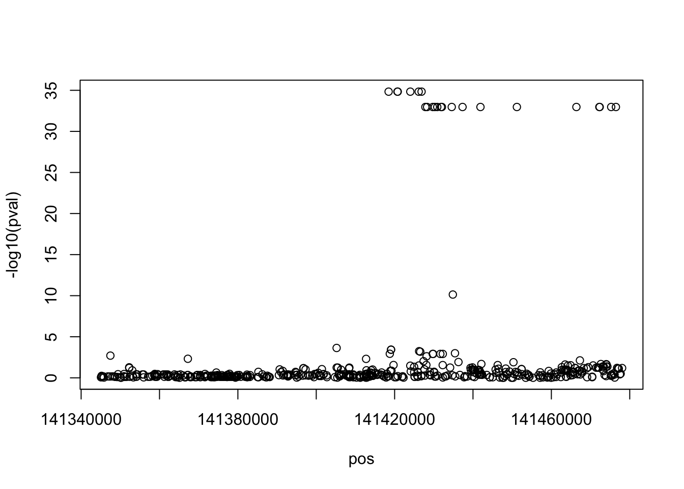
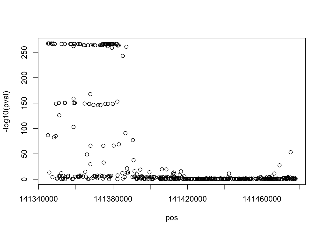
Generate summary statistics for a single causal variant and
set.seed (1234 )<- map$ map %>% generate_gwas_params (h2= 0.003 , Pi= 1 / nrow (.)) %>% generate_gwas_ss (50000 , ld= map$ ld)table (ss$ beta == 0 )
plot (- log10 (pval) ~ pos, ss)
Run SuSiE
<- susie_rss (ss$ bhat / ss$ se, R = map$ ld, n = 50000 , bhat = ss$ bhat, var_y= 1 )
WARNING: XtX is not symmetric; forcing XtX to be symmetric by replacing XtX with (XtX + t(XtX))/2
Variables in credible sets:

 variable variable_prob cs
      286     0.1604616  1
      306     0.1604616  1
      291     0.1604616  1
      300     0.1604616  1
      274     0.1604616  1
      284     0.1604616  1

Credible sets summary:

 cs cs_log10bf cs_avg_r2 cs_min_r2                variable
  1   30.37357         1         1 274,284,286,291,300,306
List of 18
 $ alpha                 : num [1:10, 1:501] 6.9e-35 2.0e-03 2.0e-03 2.0e-03 2.0e-03 ...
 $ mu                    : num [1:10, 1:501] 0.000761 0 0 0 0 ...
 $ mu2                   : num [1:10, 1:501] 2.04e-05 0.00 0.00 0.00 0.00 ...
 $ KL                    : num [1:10] 6.75 -1.24e-14 -1.24e-14 -1.24e-14 -1.24e-14 ...
 $ lbf                   : num [1:10] 6.99e+01 1.24e-14 1.24e-14 1.24e-14 1.24e-14 ...
 $ lbf_variable          : num [1:10, 1:501] -2.51 0 0 0 0 ...
 $ sigma2                : num 1
 $ V                     : num [1:10] 0.00307 0 0 0 0 ...
 $ pi                    : num [1:501] 0.002 0.002 0.002 0.002 0.002 ...
 $ null_index            : num 0
 $ XtXr                  : num [1:501, 1] -0.328 70.558 72.085 70.558 70.558 ...
 $ converged             : logi TRUE
 $ elbo                  : num [1:2] -70876 -70876
 $ niter                 : int 2
 $ X_column_scale_factors: num [1:501] 1 1 1 1 1 1 1 1 1 1 ...
 $ intercept             : num NA
 $ sets                  :List of 5
  ..$ cs                :List of 1
  .. ..$ L1: int [1:6] 274 284 286 291 300 306
  ..$ purity            :'data.frame':  1 obs. of  3 variables:
  .. ..$ min.abs.corr   : num 1
  .. ..$ mean.abs.corr  : num 1
  .. ..$ median.abs.corr: num 1
  ..$ cs_index          : int 1
  ..$ coverage          : num 0.963
  ..$ requested_coverage: num 0.95
 $ pip                   : num [1:501] 0 0 0 0 0 0 0 0 0 0 ...
 - attr(*, "class")= chr "susie"
Get Z scores from lbf
<- lbf_to_z_cont (sout$ lbf_variable[1 ,], 50000 , ss$ af, prior_v = 50 )
# A tibble: 501 × 5
     lbf     af     z    beta      se
   <dbl>  <dbl> <dbl>   <dbl>   <dbl>
 1 -2.51 0.373   1.41 0.00919 0.00654
 2 -2.43 0.169   1.37 0.0115  0.00844
 3 -2.37 0.17    1.42 0.0119  0.00842
 4 -2.43 0.169   1.37 0.0115  0.00844
 5 -2.43 0.169   1.37 0.0115  0.00844
 6 -2.52 0.191   1.32 0.0106  0.00805
 7 -2.43 0.169   1.37 0.0115  0.00844
 8 -2.44 0.17    1.36 0.0115  0.00842
 9  2.23 0.0139  3.17 0.0855  0.0270
10 -2.43 0.169   1.37 0.0115  0.00844
# … with 491 more rows
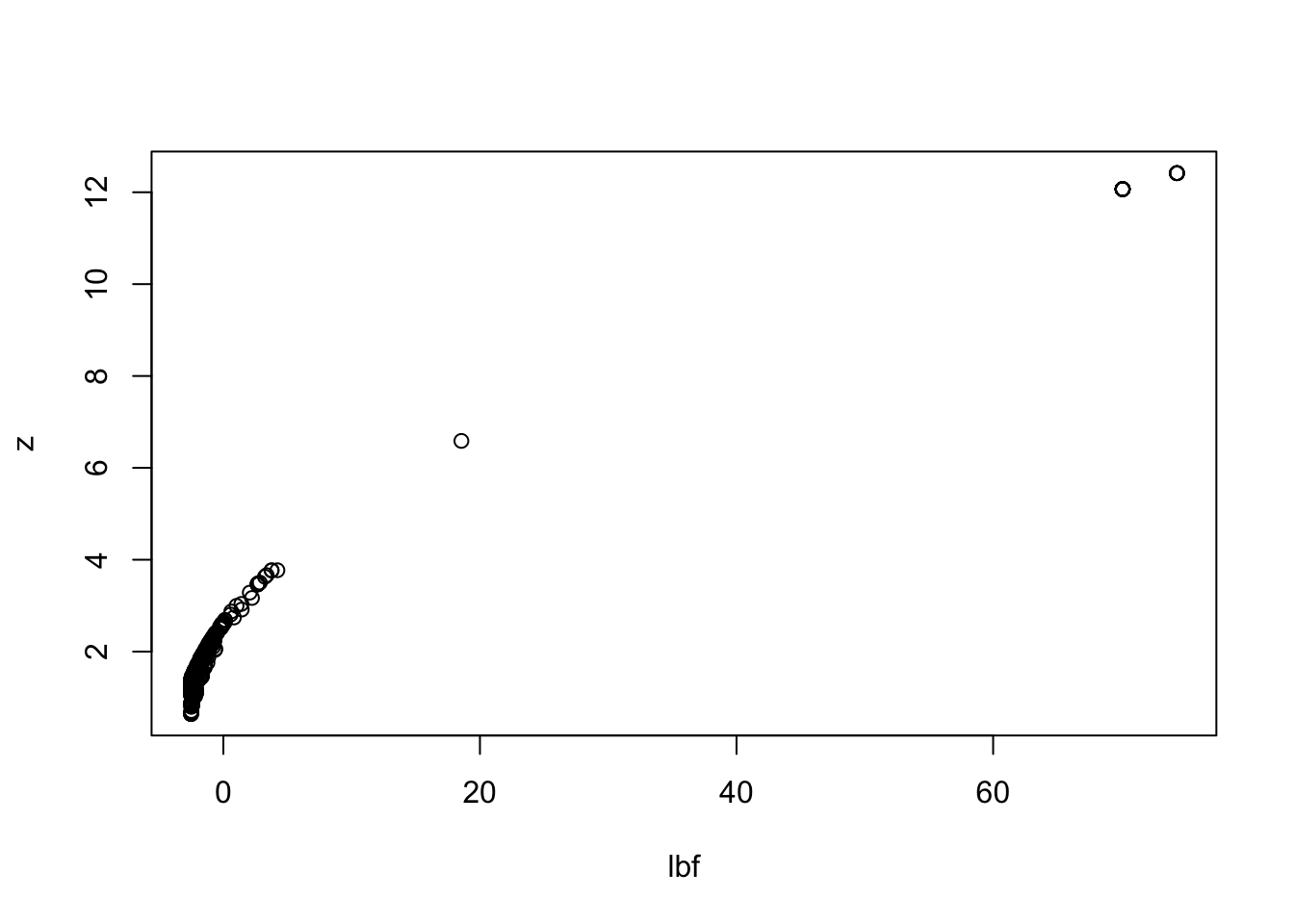
Relationship between lbf and re-estimated z
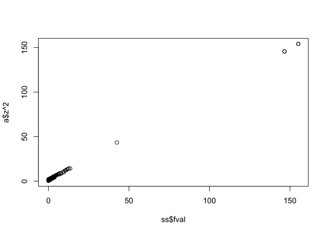
New Z vs original Z
Call:
lm(formula = a$z^2 ~ ss$fval)

Coefficients:
(Intercept)      ss$fval
     1.5141       0.9834
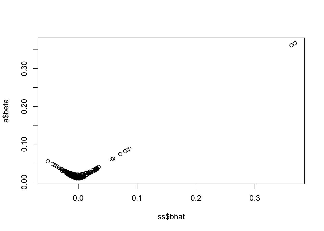
New beta vs original beta
Two causal variants
Set two causal variants at either end of the region
set.seed (12 )<- map$ map$ beta <- 0 $ beta[c (10 , 490 )] <- 0.3 <- generate_gwas_ss (param, 50000 , ld= map$ ld)plot (- log10 (pval) ~ pos, ss)
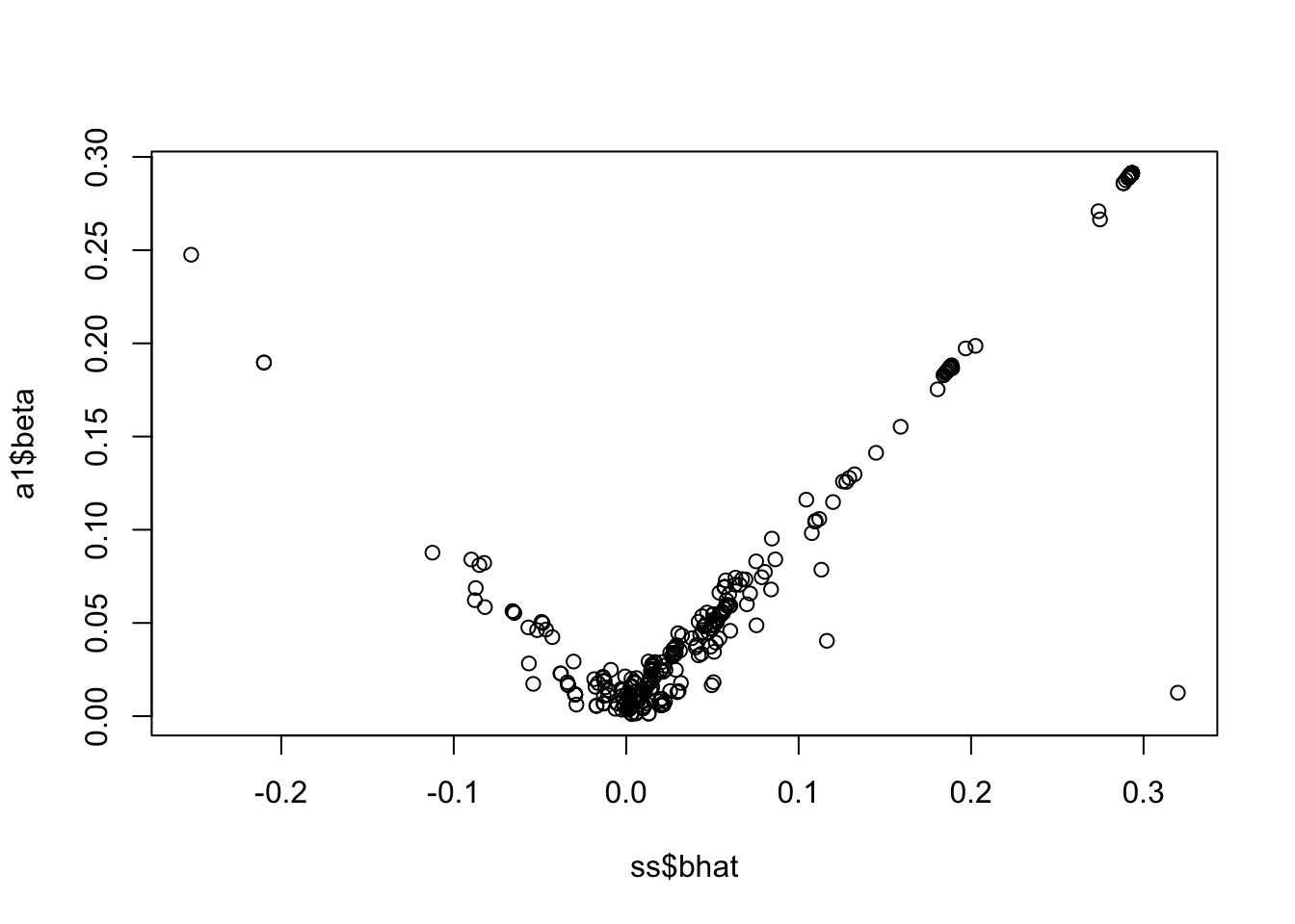
First variant
<- susie_rss (ss$ bhat / ss$ se, R = map$ ld, n = 50000 , bhat = ss$ bhat, var_y= 1 )
WARNING: XtX is not symmetric; forcing XtX to be symmetric by replacing XtX with (XtX + t(XtX))/2
<- lbf_to_z_cont (sout$ lbf_variable[1 ,], 50000 , ss$ af, prior_v = 50 )
Warning in sqrt((2 * lbf - log(sqrt(1 - r)))/r): NaNs produced
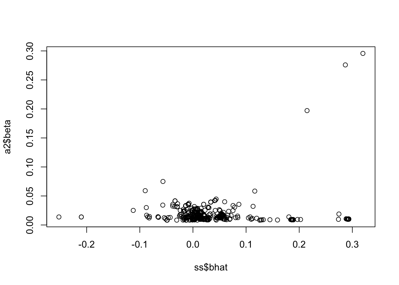
<- lbf_to_z_cont (sout$ lbf_variable[2 ,], 50000 , ss$ af, prior_v = 50 )plot (a2$ beta ~ ss$ bhat)
This looks good - it’s setting different values to 0 in the two lbf vectors that correspond to two causal variants
R version 4.2.1 Patched (2022-09-06 r82817)
Platform: aarch64-apple-darwin20 (64-bit)
Running under: macOS Monterey 12.6.2

Matrix products: default
BLAS:   /Library/Frameworks/R.framework/Versions/4.2-arm64/Resources/lib/libRblas.0.dylib
LAPACK: /Library/Frameworks/R.framework/Versions/4.2-arm64/Resources/lib/libRlapack.dylib

locale:
[1] en_GB.UTF-8/en_GB.UTF-8/en_GB.UTF-8/C/en_GB.UTF-8/en_GB.UTF-8

attached base packages:
[1] stats     graphics  grDevices utils     datasets  methods   base

other attached packages:
[1] dplyr_1.0.10     here_1.0.1       susieR_0.12.27   simulateGP_0.1.2

loaded via a namespace (and not attached):
 [1] Rcpp_1.0.9         plyr_1.8.7         compiler_4.2.1     pillar_1.8.1
 [5] tools_4.2.1        digest_0.6.31      jsonlite_1.8.4     evaluate_0.19
 [9] lifecycle_1.0.3    tibble_3.1.8       gtable_0.3.1       lattice_0.20-45
[13] pkgconfig_2.0.3    rlang_1.0.6        Matrix_1.4-1       DBI_1.1.3
[17] cli_3.5.0          yaml_2.3.6         xfun_0.36          fastmap_1.1.0
[21] stringr_1.5.0      knitr_1.41         generics_0.1.3     vctrs_0.5.1
[25] htmlwidgets_1.5.4  rprojroot_2.0.3    tidyselect_1.2.0   grid_4.2.1
[29] reshape_0.8.9      glue_1.6.2         R6_2.5.1           fansi_1.0.3
[33] rmarkdown_2.16     mixsqp_0.3-48      irlba_2.3.5.1      ggplot2_3.4.0
[37] magrittr_2.0.3     MASS_7.3-58.1      matrixStats_0.63.0 scales_1.2.1
[41] htmltools_0.5.4    assertthat_0.2.1   colorspace_2.0-3   utf8_1.2.2
[45] stringi_1.7.8      munsell_0.5.0      crayon_1.5.2