Objective
Backman et al 2022 (https://www.nature.com/articles/s41586-021-04103-z) performed exome GWAS of 4k traits, and found 564 rare-variant - trait pairs. They corrected for 20 PCs from common variants and 20 PCs from rare variants.
Question: Is uncontrolled recent population stratification biasing these associations or even driving false positives?
We could use siblings to estimate the direct effects for these discovery associations. There would be two major hits to power, first only 20k of the 500k UK Biobank will be used. Second, power to detect direct effects using siblings is reduced. So we can’t conclude that these are false positives if they simply don’t replicate in the sibling analysis.
Instead, we can ask to what extent are the replication associations consistent with the original estimates, given the reduction in precision. i.e. What fraction are expected to replicate at some nominal threshold, and what fraction are observed to replicate. If there is a significant difference between the observed and expected replication rate, then that indicates uncorrected inflation in the discovery exome GWAS.
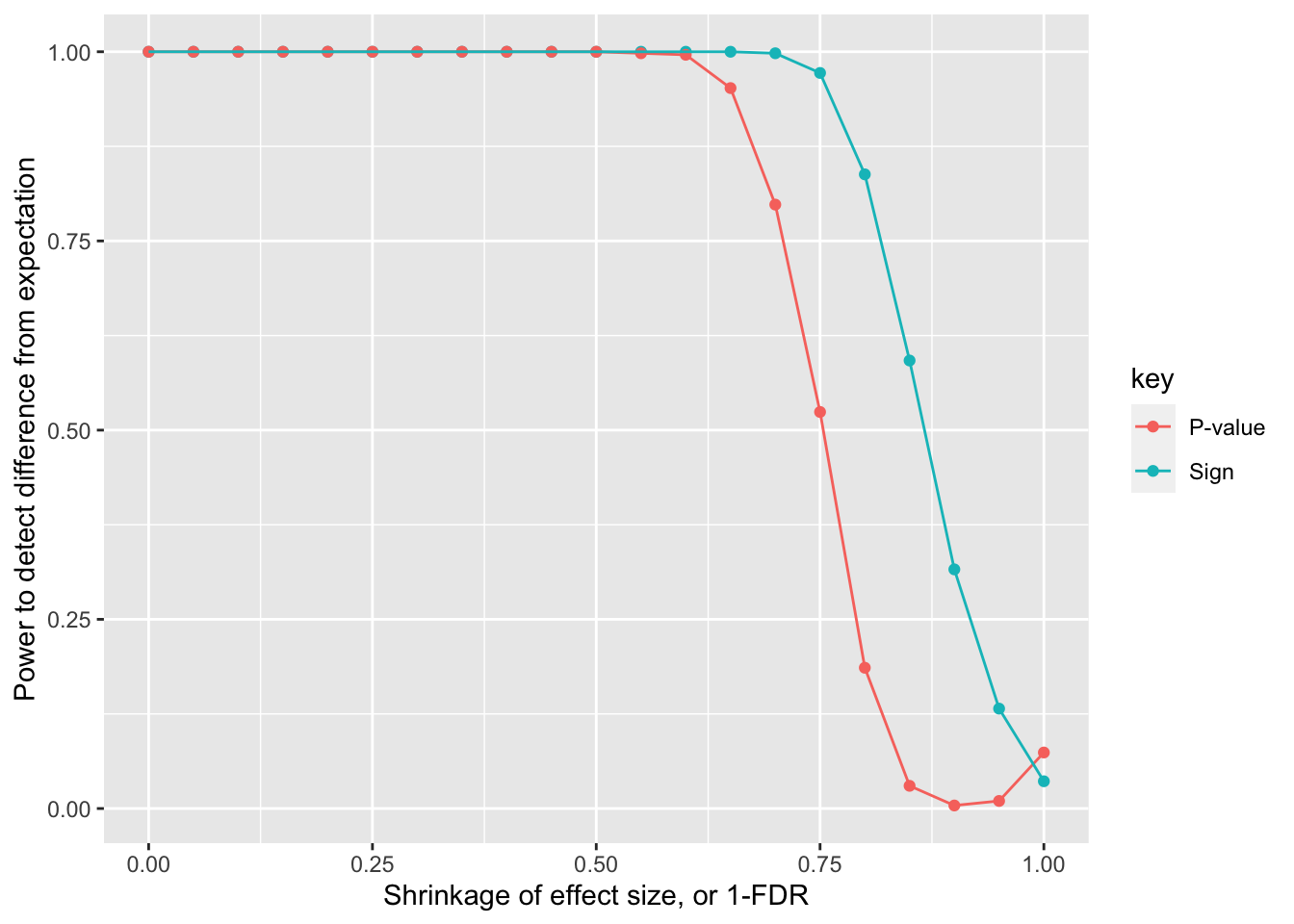
This analysis: Power calculation - how much shrinkage would there need to be before there is 80% power to detect a difference between the sibling estimate and the population estimate?
Read in Backman results
There were 564 rare-variant - trait pairs in Backman et al 2022. Of these 484 were for quantitative traits, restricting to those here for simplicity.
here() starts at /Users/gh13047/repo/lab-book
Attaching package: 'dplyr'
The following objects are masked from 'package:stats':

    filter, lag
The following objects are masked from 'package:base':

    intersect, setdiff, setequal, union
library (ggplot2)set.seed (12345 )<- read.csv ("Book3.csv" , stringsAsFactors= FALSE , header= TRUE ) %>% as_tibble () %>% mutate (se = (uci - beta)/ 1.96 )%>% glimpse ()
Rows: 484
Columns: 14
$ Effect..95..CI. <chr> "-0.15 (-0.19, -0.11)", …
$ P.value <dbl> 9.25e-12, 1.24e-24, 1.03…
$ Effect.direction <chr> "-", "-", "-", "+", "-",…
$ N.cases.with.0.1.2.copies.of.effect.allele <chr> "88038|1684|13", "418277…
$ N.controls.with.0.1.2.copies.of.effect.allele <chr> "NA|NA|NA", "NA|NA|NA", …
$ Effect.allele.frequency <dbl> 9.5e-03, 2.1e-04, 4.9e-0…
$ AA <int> 88038, 418277, 407938, 3…
$ AB <int> 1684, 177, 4027, 4076, 1…
$ BB <int> 13, 0, 11, 1, 8, 0, 1, 0…
$ N <int> 89735, 418454, 411976, 3…
$ beta <dbl> -0.150, -0.720, -0.100, …
$ lci <chr> "-0.19", "-0.86", "-0.13…
$ uci <dbl> -0.110, -0.580, -0.079, …
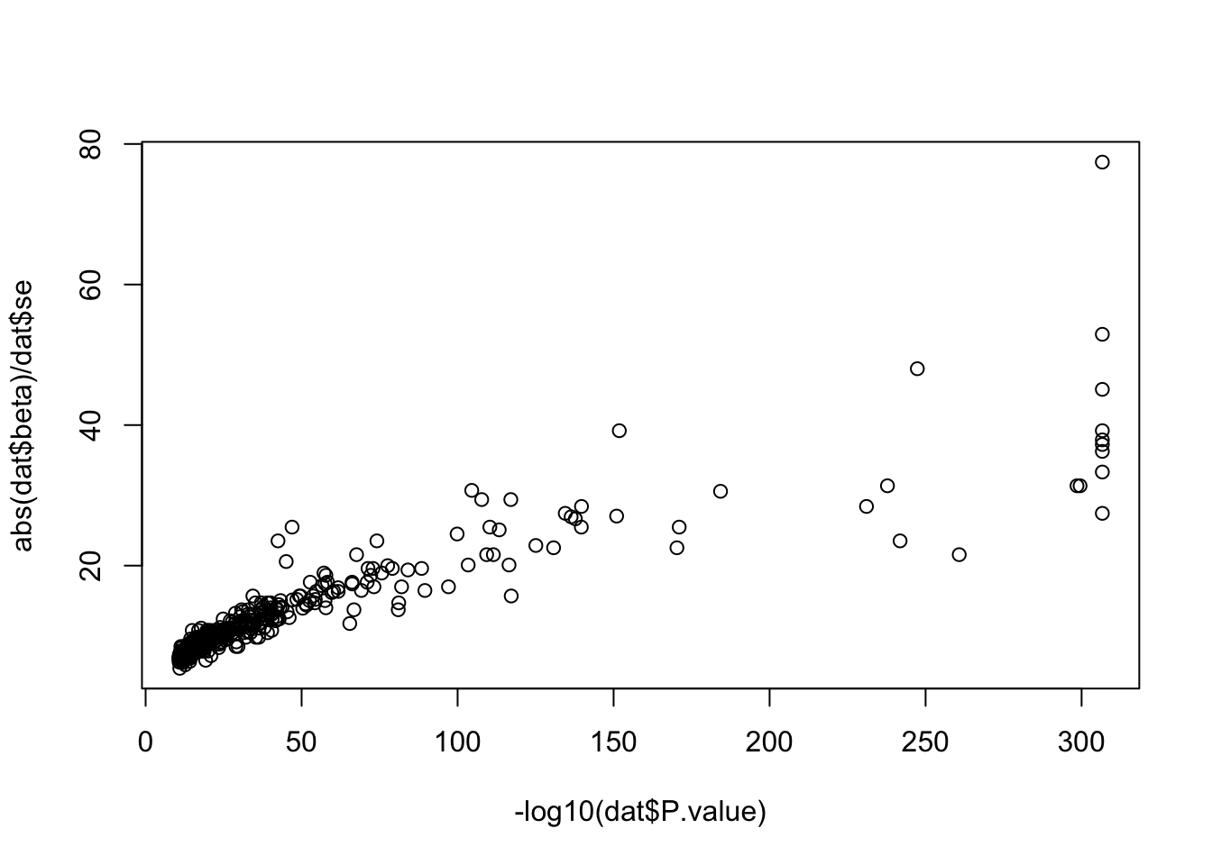
$ se <dbl> 0.020408163, 0.071428571…
plot (- log10 (dat$ P.value), abs (dat$ beta)/ dat$ se)
Functions from Alex for relative sample size between designs:
= function (h2){return (1 + h2* (1 - h2)/ (4 - h2))= function (h2){return ((1 + h2* (1 - h2)/ (4 - h2))^ (- 1 ))= function (h2){return (1 + h2* (1 - h2)/ (3 - h2* (1 + h2/ 2 )))= function (h2){return ((1 + h2* (1 - h2)/ (3 - h2* (1 + h2/ 2 )))^ (- 1 ))= function (h2){return (0.5 / 3 )}= function (h2){return ((2 * (2 - h2))^ (- 1 ))}= function (h2){return ((2 + h2/ 2 )/ (6 * (1 - (h2/ 2 )^ 2 )))}
Function to estimate expected replication rate
<- function (b_disc, b_rep, se_disc, se_rep, alpha)<- pnorm (- abs (b_disc) / se_disc) * pnorm (- abs (b_disc) / se_rep) + ((1 - pnorm (- abs (b_disc) / se_disc)) * (1 - pnorm (- abs (b_disc) / se_rep)))<- pnorm (- abs (b_disc) / se_rep + qnorm (alpha / 2 )) + (1 - pnorm (- abs (b_disc) / se_rep - qnorm (alpha / 2 )))<- pnorm (abs (b_rep)/ se_rep, lower.tail= FALSE )<- tibble:: tibble (nsnp= length (b_disc),metric= c ("Sign" , "Sign" , "P-value" , "P-value" ),datum= c ("Expected" , "Observed" , "Expected" , "Observed" ),value= c (sum (p_sign, na.rm= TRUE ), sum (sign (b_disc) == sign (b_rep)), sum (p_sig, na.rm= TRUE ), sum (p_rep < alpha, na.rm= TRUE ))<- list (Sign = binom.test (res$ value[2 ], res$ nsnp[1 ], res$ value[1 ] / res$ nsnp[1 ])$ p.value,` P-value ` = binom.test (res$ value[4 ], res$ nsnp[1 ], res$ value[3 ] / res$ nsnp[1 ])$ p.value%>% as_tibble ()return (list (res= res, pdif= pdif, variants= dplyr:: tibble (sig= p_sig, sign= p_sign)))
Function to simulate assocs in siblings
<- function (beta, af, n, vy) sqrt (c (vy) - beta^ 2 * 2 * af * (1 - af))/ sqrt (n) * (1 / sqrt (2 * * (1 - af)))<- function (beta, af, n, se)^ 2 * 2 * af * (1 - af)* n + beta^ 2 * 2 * af * (1 - af)# check algebra! # expected_se(0.2, 0.4, 1000, 10) # expected_vy(0.2, 0.4, 1000, expected_se(0.2, 0.4, 1000, 10)) <- function (beta_disc, se_disc, af_disc, n_disc, prop_sibs, h2, alpha, shrinkage)<- tibble (beta_disc = beta_disc,beta_true = beta_disc * shrinkage,vy = expected_vy (beta_disc, af_disc, n_disc, se_disc),n_rep = n_disc * prop_sibs * unrel_vs_direct_sibimp (h2),se_rep = expected_se (beta_disc, af_disc, n_rep, vy),beta_rep = rnorm (length (beta_disc), beta_true, se_rep)%>% prop_overlap (.$ beta_disc, .$ beta_rep, se_disc, .$ se_rep, alpha)}
Power analysis
<- expand.grid (sim= 1 : 500 , shrinkage= seq (0 ,1 ,0.05 ))<- lapply (1 : nrow (params), function (i) simgwas_sib (dat$ beta, dat$ se, dat$ Effect.allele.frequency, dat$ N, 20000 / 500000 ,0.5 , 0.05 / nrow (dat), params$ shrinkage[i])%>% lapply (., function (x) x$ pdif) %>% bind_rows () %>% bind_cols (., params)
# A tibble: 10,500 × 4
        Sign `P-value`   sim shrinkage
       <dbl>     <dbl> <int>     <dbl>
 1 1.04e- 91  2.33e-11     1         0
 2 3.19e- 95  2.33e-11     2         0
 3 7.72e- 91  2.33e-11     3         0
 4 4.13e- 89  2.33e-11     4         0
 5 3.52e-105  2.33e-11     5         0
 6 6.78e- 98  2.33e-11     6         0
 7 1.85e- 93  2.33e-11     7         0
 8 4.14e- 96  2.33e-11     8         0
 9 1.76e-118  9.03e-10     9         0
10 9.63e-112  2.33e-11    10         0
# … with 10,490 more rows
%>% group_by (shrinkage) %>% summarise (Sign= sum (Sign < 0.05 )/ n (), ` P-value ` = sum (` P-value ` < 0.05 )/ n ()) %>% :: gather (key= "key" , value= "value" , c (` Sign ` , ` P-value ` )) %>% ggplot (., aes (x= shrinkage, y= value)) + geom_point (aes (colour= key)) + geom_line (aes (colour= key)) + labs (x= "Shrinkage of effect size, or 1-FDR" , y= "Power to detect difference from expectation" )
Summary
Power is quite high to detect a difference!
R version 4.2.1 Patched (2022-09-06 r82817)
Platform: aarch64-apple-darwin20 (64-bit)
Running under: macOS Monterey 12.6.2

Matrix products: default
BLAS:   /Library/Frameworks/R.framework/Versions/4.2-arm64/Resources/lib/libRblas.0.dylib
LAPACK: /Library/Frameworks/R.framework/Versions/4.2-arm64/Resources/lib/libRlapack.dylib

locale:
[1] en_GB.UTF-8/en_GB.UTF-8/en_GB.UTF-8/C/en_GB.UTF-8/en_GB.UTF-8

attached base packages:
[1] stats     graphics  grDevices utils     datasets  methods   base

other attached packages:
[1] ggplot2_3.4.0 dplyr_1.0.10  here_1.0.1

loaded via a namespace (and not attached):
 [1] pillar_1.8.1      compiler_4.2.1    tools_4.2.1       digest_0.6.31
 [5] jsonlite_1.8.4    evaluate_0.19     lifecycle_1.0.3   tibble_3.1.8
 [9] gtable_0.3.1      pkgconfig_2.0.3   rlang_1.0.6       cli_3.5.0
[13] DBI_1.1.3         yaml_2.3.6        xfun_0.36         fastmap_1.1.0
[17] withr_2.5.0       stringr_1.5.0     knitr_1.41        generics_0.1.3
[21] vctrs_0.5.1       htmlwidgets_1.5.4 rprojroot_2.0.3   grid_4.2.1
[25] tidyselect_1.2.0  glue_1.6.2        R6_2.5.1          fansi_1.0.3
[29] rmarkdown_2.16    farver_2.1.1      tidyr_1.2.1       purrr_1.0.0
[33] magrittr_2.0.3    ellipsis_0.3.2    scales_1.2.1      htmltools_0.5.4
[37] assertthat_0.2.1  colorspace_2.0-3  labeling_0.4.2    utf8_1.2.2
[41] stringi_1.7.8     munsell_0.5.0