Probability of a random variable being larger than all other random variables in a multivariate normal vector

I have 1k SNPs in a region. I know the causal variant and the LD matrix. The effect size at each SNP will be related to the allele frequency and the LD at all other variants. The SE across the SNPs will be correlated in relation to the LD. I can generate the expected effect size and the variance covariance matrix of the effects. Once I have that, I can generate beta values from a multivariate normal distribution, and determine how often each of the SNPs is the top SNP.

Is there a faster way to do this by getting the probability from a multivariate normal distribution?

Related to this question: https://stats.stackexchange.com/a/4181

library(MCMCpack)

Loading required package: coda

Loading required package: MASS

##
## Markov Chain Monte Carlo Package (MCMCpack)

## Copyright (C) 2003-2022 Andrew D. Martin, Kevin M. Quinn, and Jong Hee Park

##
## Support provided by the U.S. National Science Foundation

## (Grants SES-0350646 and SES-0350613)
##

library(dplyr)

Attaching package: 'dplyr'

The following object is masked from 'package:MASS':

    select

The following objects are masked from 'package:stats':

    filter, lag

The following objects are masked from 'package:base':

    intersect, setdiff, setequal, union

library(simulateGP)
library(MASS)
library(mvtnorm)

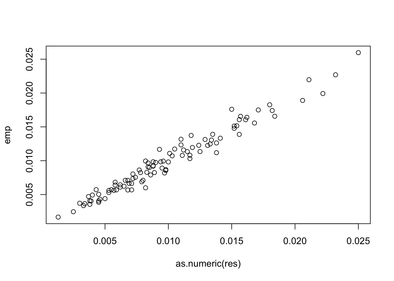
Empirical simulation for probabilities, case of 3 variables

n <- 3
mu <- rnorm(n)
S <- rwish(n, diag(n))
emp <- mvrnorm(1000, mu, S)
res <- apply(emp, 1, function(x) which.max(x)) %>% table() %>% prop.table()
res

.
    1     2     3 
0.666 0.146 0.188 

A <- matrix(c(1,-1,0, 1,0,-1), nrow = 2, byrow = TRUE)
newMu <- as.vector(A %*% mu)
newS <- A %*% S %*% t(A)
pmvnorm(lower=c(0,0), mean = newMu, sigma = newS)

[1] 0.6660382
attr(,"error")
[1] 1e-15
attr(,"msg")
[1] "Normal Completion"

A <- matrix(c(1,-1,0, 1,0,-1), nrow = 2, byrow = TRUE)
A <- A[,c(2,1,3)]
newMu <- as.vector(A %*% mu)
newS <- A %*% S %*% t(A)
pmvnorm(lower=c(0,0), mean = newMu, sigma = newS)

[1] 0.1487365
attr(,"error")
[1] 1e-15
attr(,"msg")
[1] "Normal Completion"

A <- matrix(c(1,-1,0, 1,0,-1), nrow = 2, byrow = TRUE)
A <- A[,c(2,3,1)]
newMu <- as.vector(A %*% mu)
newS <- A %*% S %*% t(A)
pmvnorm(lower=c(0,0), mean = newMu, sigma = newS)

[1] 0.1852253
attr(,"error")
[1] 1e-15
attr(,"msg")
[1] "Normal Completion"

Increase to arbitrary variables

Use wishart distribution to generate random vcov matrix

n <- 100
mu <- rnorm(n)
S <- rwish(n, diag(n))

Empirically generate correlated variables and count how often each one is the largest

samp <- mvrnorm(10000, mu, S)
res <- apply(samp, 1, function(x) which.max(x)) %>% table() %>% prop.table()
res

.
     1      2      3      4      5      6      7      8      9     10     11 
0.0232 0.0085 0.0211 0.0072 0.0152 0.0118 0.0038 0.0161 0.0058 0.0094 0.0080 
    12     13     14     15     16     17     18     19     20     21     22 
0.0083 0.0152 0.0250 0.0103 0.0131 0.0115 0.0112 0.0093 0.0105 0.0084 0.0066 
    23     24     25     26     27     28     29     30     31     32     33 
0.0055 0.0088 0.0150 0.0098 0.0182 0.0171 0.0065 0.0090 0.0074 0.0134 0.0057 
    34     35     36     37     38     39     40     41     42     43     44 
0.0125 0.0084 0.0129 0.0088 0.0110 0.0222 0.0154 0.0079 0.0046 0.0111 0.0045 
    45     46     47     48     49     50     51     52     53     54     55 
0.0045 0.0071 0.0034 0.0045 0.0133 0.0053 0.0096 0.0013 0.0078 0.0138 0.0053 
    56     57     58     59     60     61     62     63     64     65     66 
0.0138 0.0039 0.0025 0.0101 0.0100 0.0059 0.0050 0.0206 0.0043 0.0157 0.0068 
    67     68     69     70     71     72     73     74     75     76     77 
0.0068 0.0119 0.0097 0.0117 0.0030 0.0162 0.0082 0.0040 0.0077 0.0156 0.0037 
    78     79     80     81     82     83     84     85     86     87     88 
0.0135 0.0082 0.0168 0.0033 0.0095 0.0072 0.0062 0.0124 0.0062 0.0156 0.0088 
    89     90     91     92     93     94     95     96     97     98     99 
0.0038 0.0141 0.0086 0.0089 0.0184 0.0117 0.0069 0.0180 0.0098 0.0110 0.0058 
   100 
0.0071 

Use probability density function instead, evaluating for each variable the probability that it’s larger than all the other variables

# Create design matrix
swap_1 <- function(n, i)
{
  ind <- 1:n
  if(i == 1) return(ind)
  ind[i] <- 1
  ind[1:(i-1)] <- 2:i
  return(ind)
}
#sapply(1:7, function(i) swap_1(7, i))
A <- cbind(
  rep(1, n-1),
  diag(rep(-1, n-1))
) %>% as.matrix()

emp <- sapply(1:n, function(i)
{
  A <- A[,swap_1(n,i)]
  newMu <- as.vector(A %*% mu)
  newS <- A %*% S %*% t(A)
  pmvnorm(lower=rep(0,n-1), mean = newMu, sigma = newS)
})
plot(emp ~ as.numeric(res))

Theoretical result works fine but is slower than empirical sampling.