Power of GWAS in ascertained case control datasets

Case control studies ascertain a fixed number of cases and controls. This changes the distribution of genetic liability in the selected sample - e.g. if the prevalence is low then the liability will be a truncated distribution for cases ascertained for the tail of the distribution, and truncated for the controls ascertained for a depletion of values in the tail (e.g. see here for illustrations https://pubmed.ncbi.nlm.nih.gov/21376301/).

The more rare the disease, the larger the variance of the liability when cases and controls are matched. This should improve statistical power because the cases and controls are ascertained to be more genetically distinct from each other.

However, the Genetic Power Calculator concludes the opposite, as prevalence gets lower the power goes down (https://zzz.bwh.harvard.edu/gpc/cc2.html). e.g. for OR=1.1, ncase=1000, ncontrol=1000, af=0.5, for 80% power:

• prev = 0.001, power = 4e-5
• prev = 0.4, power = 0.71

Quick simulation to investigate:

library(simulateGP)
library(dplyr)

Attaching package: 'dplyr'

The following objects are masked from 'package:stats':

    filter, lag

The following objects are masked from 'package:base':

    intersect, setdiff, setequal, union

library(ggplot2)

Generate a function that will

1. create a population with some genetic liability
2. stochastically assign disease status based on heritability and prevalence
3. ascertain cases and controls
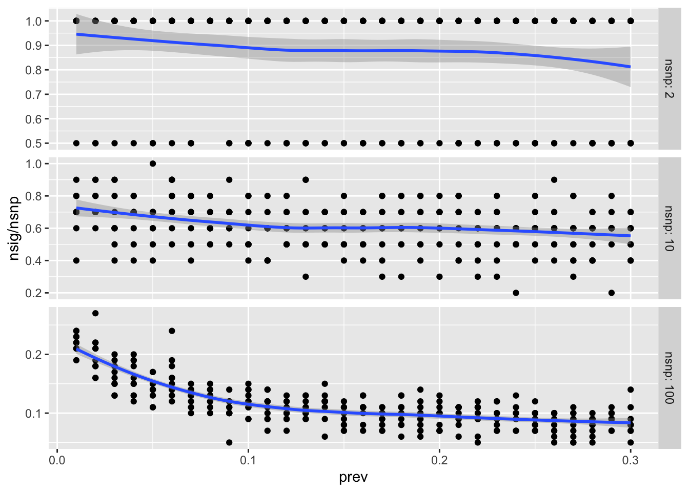
4. identify how many significant associations in the case/control sample

sims <- function(ncase, ncontrol, nsnp, prev, hsq=0.5, thresh=5e-8)
{
  # Determine minimum sample size required to ascertain required number of cases and controls
  n_req <- round(max(ncase / prev, ncontrol / prev) + 10000)
  
  # Generate matrix of genotype values
  g <- make_geno(n_req, nsnp, 0.5)
  
  # Effect sizes for each SNP
  b <- rnorm(nsnp)

  dat <- tibble(
    id = 1:n_req,
    l = scale(g %*% b),               # genetic liability
    p = gx_to_gp(l, hsq, prev),       # convert to disease probability
    d = rbinom(n_req, 1, p)           # sample disease status from probability
  )
  
  # Ascertain cases and controls 
  dat <- rbind(
    subset(dat, d == 0)[1:ncase,],
    subset(dat, d == 1)[1:ncontrol,]
  )

  # Perform GWAS
  res <- gwas(dat$d, g[dat$id,], logistic=TRUE)
  
  # Count number of significant assocs
  return(sum(res$pval < thresh))
}

Run a bunch of simulations

params <- expand.grid(
  ncase = 1000,
  ncontrol = 1000, 
  nsnp = c(2, 10, 100),
  repeats = 1:10,
  prev = seq(0.01, 0.3, by=0.01),
  hsq=0.5,
  thresh=5e-8
) %>% select(-repeats)
params$nsig <- sapply(1:nrow(params), function(i) do.call(sims, params[i,]))

Plot

ggplot(params, aes(x=prev, y=nsig/nsnp)) +
  geom_point() +
  facet_grid(nsnp ~ ., labeller=label_both, scale="free_y") +
  geom_smooth()

`geom_smooth()` using method = 'loess' and formula = 'y ~ x'

So power increases when prevalence is lower. Maybe this is related to polygenicity.

So what’s GPC doing differently to get the opposite result (lower prev = lower power)?