Gibran Hemani’s lab book

How does PRS compare to IVW fixed effects analysis

Simulation study

library(simulateGP)
geno1 <- make_geno(10000, 500, 0.5)
b <- choose_effects(500, 0.3)
x1 <- make_phen(b, geno1)
y1 <- make_phen(0.4, x1)

geno2 <- make_geno(1000, 500, 0.5)
x2 <- make_phen(b, geno2)
y2 <- make_phen(0.4, x2)

bhat <- gwas(x1, geno1)
b_unweighted <- sign(b)

Standard unweighted PRS analysis

prs_unweighted <- geno2 %*% b_unweighted
summary(lm(x2 ~ prs_unweighted))


Call:
lm(formula = x2 ~ prs_unweighted)

Residuals:
    Min      1Q  Median      3Q     Max 
-3.2356 -0.5547 -0.0330  0.6087  3.1932 

Coefficients:
                Estimate Std. Error t value Pr(>|t|)    
(Intercept)    -0.321168   0.035444  -9.061   <2e-16 ***
prs_unweighted  0.027292   0.001791  15.239   <2e-16 ***
---
Signif. codes:  0 '***' 0.001 '**' 0.01 '*' 0.05 '.' 0.1 ' ' 1

Residual standard error: 0.9011 on 998 degrees of freedom
Multiple R-squared:  0.1888,    Adjusted R-squared:  0.1879 
F-statistic: 232.2 on 1 and 998 DF,  p-value: < 2.2e-16

Meta analysing per-SNP PRS scores

library(meta)

Loading 'meta' package (version 6.0-0).
Type 'help(meta)' for a brief overview.
Readers of 'Meta-Analysis with R (Use R!)' should install
older version of 'meta' package: https://tinyurl.com/dt4y5drs

o <- sapply(1:ncol(geno2), function(i)
{
  prs_unweighted <- geno2[,i] * b_unweighted[i]
  summary(lm(x2 ~ prs_unweighted))$coef[2,1:2]
})
metafor::rma(yi=o[1,], sei=o[2,], method="EE")


Equal-Effects Model (k = 500)

I^2 (total heterogeneity / total variability):   17.58%
H^2 (total variability / sampling variability):  1.21

Test for Heterogeneity:
Q(df = 499) = 605.4622, p-val = 0.0007

Model Results:

estimate      se     zval    pval   ci.lb   ci.ub      
  0.0277  0.0020  13.8615  <.0001  0.0238  0.0316  *** 

---
Signif. codes:  0 '***' 0.001 '**' 0.01 '*' 0.05 '.' 0.1 ' ' 1

Standard errors with number of SNPs

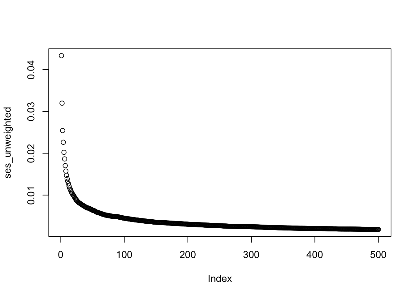
ses_unweighted <- sapply(1:ncol(geno2), function(i)
{
  prs_unweighted <- geno2[,1:i, drop=FALSE] %*% b_unweighted[1:i]
  summary(lm(x2 ~ prs_unweighted))$coef[2,2]
})
plot(ses_unweighted)